
8: Topical Overview of PIB and Postulates QM (Lecture)
- Page ID
- 198573
\( \newcommand{\vecs}[1]{\overset { \scriptstyle \rightharpoonup} {\mathbf{#1}} } \)
\( \newcommand{\vecd}[1]{\overset{-\!-\!\rightharpoonup}{\vphantom{a}\smash {#1}}} \)
\( \newcommand{\id}{\mathrm{id}}\) \( \newcommand{\Span}{\mathrm{span}}\)
( \newcommand{\kernel}{\mathrm{null}\,}\) \( \newcommand{\range}{\mathrm{range}\,}\)
\( \newcommand{\RealPart}{\mathrm{Re}}\) \( \newcommand{\ImaginaryPart}{\mathrm{Im}}\)
\( \newcommand{\Argument}{\mathrm{Arg}}\) \( \newcommand{\norm}[1]{\| #1 \|}\)
\( \newcommand{\inner}[2]{\langle #1, #2 \rangle}\)
\( \newcommand{\Span}{\mathrm{span}}\)
\( \newcommand{\id}{\mathrm{id}}\)
\( \newcommand{\Span}{\mathrm{span}}\)
\( \newcommand{\kernel}{\mathrm{null}\,}\)
\( \newcommand{\range}{\mathrm{range}\,}\)
\( \newcommand{\RealPart}{\mathrm{Re}}\)
\( \newcommand{\ImaginaryPart}{\mathrm{Im}}\)
\( \newcommand{\Argument}{\mathrm{Arg}}\)
\( \newcommand{\norm}[1]{\| #1 \|}\)
\( \newcommand{\inner}[2]{\langle #1, #2 \rangle}\)
\( \newcommand{\Span}{\mathrm{span}}\) \( \newcommand{\AA}{\unicode[.8,0]{x212B}}\)
\( \newcommand{\vectorA}[1]{\vec{#1}} % arrow\)
\( \newcommand{\vectorAt}[1]{\vec{\text{#1}}} % arrow\)
\( \newcommand{\vectorB}[1]{\overset { \scriptstyle \rightharpoonup} {\mathbf{#1}} } \)
\( \newcommand{\vectorC}[1]{\textbf{#1}} \)
\( \newcommand{\vectorD}[1]{\overrightarrow{#1}} \)
\( \newcommand{\vectorDt}[1]{\overrightarrow{\text{#1}}} \)
\( \newcommand{\vectE}[1]{\overset{-\!-\!\rightharpoonup}{\vphantom{a}\smash{\mathbf {#1}}}} \)
\( \newcommand{\vecs}[1]{\overset { \scriptstyle \rightharpoonup} {\mathbf{#1}} } \)
\( \newcommand{\vecd}[1]{\overset{-\!-\!\rightharpoonup}{\vphantom{a}\smash {#1}}} \)
\(\newcommand{\avec}{\mathbf a}\) \(\newcommand{\bvec}{\mathbf b}\) \(\newcommand{\cvec}{\mathbf c}\) \(\newcommand{\dvec}{\mathbf d}\) \(\newcommand{\dtil}{\widetilde{\mathbf d}}\) \(\newcommand{\evec}{\mathbf e}\) \(\newcommand{\fvec}{\mathbf f}\) \(\newcommand{\nvec}{\mathbf n}\) \(\newcommand{\pvec}{\mathbf p}\) \(\newcommand{\qvec}{\mathbf q}\) \(\newcommand{\svec}{\mathbf s}\) \(\newcommand{\tvec}{\mathbf t}\) \(\newcommand{\uvec}{\mathbf u}\) \(\newcommand{\vvec}{\mathbf v}\) \(\newcommand{\wvec}{\mathbf w}\) \(\newcommand{\xvec}{\mathbf x}\) \(\newcommand{\yvec}{\mathbf y}\) \(\newcommand{\zvec}{\mathbf z}\) \(\newcommand{\rvec}{\mathbf r}\) \(\newcommand{\mvec}{\mathbf m}\) \(\newcommand{\zerovec}{\mathbf 0}\) \(\newcommand{\onevec}{\mathbf 1}\) \(\newcommand{\real}{\mathbb R}\) \(\newcommand{\twovec}[2]{\left[\begin{array}{r}#1 \\ #2 \end{array}\right]}\) \(\newcommand{\ctwovec}[2]{\left[\begin{array}{c}#1 \\ #2 \end{array}\right]}\) \(\newcommand{\threevec}[3]{\left[\begin{array}{r}#1 \\ #2 \\ #3 \end{array}\right]}\) \(\newcommand{\cthreevec}[3]{\left[\begin{array}{c}#1 \\ #2 \\ #3 \end{array}\right]}\) \(\newcommand{\fourvec}[4]{\left[\begin{array}{r}#1 \\ #2 \\ #3 \\ #4 \end{array}\right]}\) \(\newcommand{\cfourvec}[4]{\left[\begin{array}{c}#1 \\ #2 \\ #3 \\ #4 \end{array}\right]}\) \(\newcommand{\fivevec}[5]{\left[\begin{array}{r}#1 \\ #2 \\ #3 \\ #4 \\ #5 \\ \end{array}\right]}\) \(\newcommand{\cfivevec}[5]{\left[\begin{array}{c}#1 \\ #2 \\ #3 \\ #4 \\ #5 \\ \end{array}\right]}\) \(\newcommand{\mattwo}[4]{\left[\begin{array}{rr}#1 \amp #2 \\ #3 \amp #4 \\ \end{array}\right]}\) \(\newcommand{\laspan}[1]{\text{Span}\{#1\}}\) \(\newcommand{\bcal}{\cal B}\) \(\newcommand{\ccal}{\cal C}\) \(\newcommand{\scal}{\cal S}\) \(\newcommand{\wcal}{\cal W}\) \(\newcommand{\ecal}{\cal E}\) \(\newcommand{\coords}[2]{\left\{#1\right\}_{#2}}\) \(\newcommand{\gray}[1]{\color{gray}{#1}}\) \(\newcommand{\lgray}[1]{\color{lightgray}{#1}}\) \(\newcommand{\rank}{\operatorname{rank}}\) \(\newcommand{\row}{\text{Row}}\) \(\newcommand{\col}{\text{Col}}\) \(\renewcommand{\row}{\text{Row}}\) \(\newcommand{\nul}{\text{Nul}}\) \(\newcommand{\var}{\text{Var}}\) \(\newcommand{\corr}{\text{corr}}\) \(\newcommand{\len}[1]{\left|#1\right|}\) \(\newcommand{\bbar}{\overline{\bvec}}\) \(\newcommand{\bhat}{\widehat{\bvec}}\) \(\newcommand{\bperp}{\bvec^\perp}\) \(\newcommand{\xhat}{\widehat{\xvec}}\) \(\newcommand{\vhat}{\widehat{\vvec}}\) \(\newcommand{\uhat}{\widehat{\uvec}}\) \(\newcommand{\what}{\widehat{\wvec}}\) \(\newcommand{\Sighat}{\widehat{\Sigma}}\) \(\newcommand{\lt}{<}\) \(\newcommand{\gt}{>}\) \(\newcommand{\amp}{&}\) \(\definecolor{fillinmathshade}{gray}{0.9}\)Overview of Lecture 7:
Conceptually, applying operator \(\hat{A}\) to an eigenfunction such as \(\psi (x)\) gives an eigenvalue \(a\) back, multiplied by the same eigenfunction. Mathematically, this looks like
\[\hat{A}\psi (x) = a\psi (x) \nonumber\]
Example of operators:
Wavefunctions have a probabilistic interpretation. More specifically, the wavefunction squared (or to be more exact, the \(\Psi^*\Psi\) is a probability density). To get a probability, we have to integrate \(\psi^*\psi\) over an interval. We can never discuss the probability at one point, except in a relative fashion or if we are referring to a node (where it will never be found). The probabilistic interpretation comes with key features of \(\psi^*\psi\) including finite, nonnegative and not infinite. A key aspect of this is that the wavefunctions must be normalized.
We introduced the particle in the box, which is arguable the mode important "trapped" particle system. This system is "easy" to solve the Schrödinger Equation to get oscillatory wavefunctions.
The Particle in a one Dimensional box (a Trapped Particle)
The particle in the box model system is the simplest non-trivial application of the Schrödinger equation, but one which illustrates many of the fundamental concepts of quantum mechanics. For a particle moving in one dimension (again along the x- axis), the Schrödinger equation can be written
\[-\dfrac{\hbar^2}{2m}\psi {}''(x)+ V (x)\psi (x) = E \psi (x)\label{3.5.1}\]
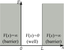
Assume that the particle can move freely between two endpoints \(x = 0\) and \(x = L\), but cannot penetrate past either end. This is equivalent to a potential energy dependent on x with
\[V(x)=\begin{cases}
0 & 0\leq x\leq L \\
\infty & x< 0 \; and\; x> L \end{cases}\label{3.5.2}\]
This potential is represented by the dark lines in Figure \(\ref{3.5.1}\). The infinite potential energy constitutes an impenetrable barrier since the particle would have an infinite potential energy if found there, which is clearly impossible.
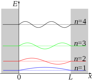
The particle in a one-dimensional box is not a real system. As seen before with vibrating strings in the classical wave function, \( X(x) = A\sin(kx)\psi (x)\). In this system, solving the Schrödinger equation (Equation \ref{3.5.1}) results in this solution:
\[ \color{red} {\psi (x) = N\sin \left(\dfrac{n\pi x}{L}\right)} \label{1a}\]
for
\[0 \leq x \leq L \label{1b}\]
with \(N\) is an arbitrary Normalization constant.
Since a particle cannot have infinite energy, it cannot exist outside the box (Equation \ref{3.5.2}) and furthermore, two Boundary conditions are therefore expected:
\[\begin{align} \psi (x=0) = 0 \label{3.5.3A1} \\[4pt] \psi (x=L) = 0 \label{3.5.3A2} \end{align}\]
This results in the quantization in allowed levels. For the one dimensional box, the eigenvalue is
\[ \color{red} {E_n = \dfrac{h^2 n^2 }{8m_e L^2}} \label{3.5.11}\]
These are the only values of the energy which allows solutions of the Schrödinger Equation \(\ref{3.5.1}\) consistent with the boundary conditions in Equations \ref{3.5.3A1} and \ref{3.5.3A2}. The integer \(n\) in Equation \ref{1a} is called a quantum number, is appended as a subscript on \(E\) to label the allowed energy levels. Negative values of \(n\) add nothing new because the energies in Equation \ref{3.5.11} depends on \(n^2\).
Transition from one Eigenstate to another
Like the hydrogen atom, you can figure out the spectrum for transitions from \(n_1\) to \(n_2\) by the standard spectroscopy equation (i.e., conservation of energy)
\[\Delta E = E_{n_2} - E_{n_1} = hc/\lambda \nonumber\]
Normalize the Wavefunction
To normalize the wave function \(\psi (x)\) it is important to recognize that \(\int_{-\infty}^{\infty} \psi_n^* \psi_n dx\) is the probability of finding a particle in all space, which is 1, or 100%. The integral can be broken up into three parts, defined by the system's boundary conditions:
\[\int_{-\infty}^{0} \psi_n^* \psi_n dx+ \int_{0}^{L} \psi_n^* \psi_n dx + \int_{L}^{\infty} \psi_n^* \psi_n dx = 1 \label{PIB2}\]
since \(\psi (x) = 0\) when \(x<0\) and \(x>a\), the first and last integral of the summation of integrals are zero. That leaves \(N^2\int_{0}^{L} \psi_n^* \psi_n dx\ = 1\), where \(N\) is the normalization constant. Thus,
\[1=N^2 \int_0^L {\sin}^2(n\pi x/L)dx = N^2(L/2) \label{PIB3}.\]
Solving for \(N\) = \(\sqrt{2/L}\). Going back to \(\psi (x) = B\sin(\frac {n\pi x}{a})\), the new equation becomes
\[ \color{red} {\psi (x) = \sqrt{\frac{2}{L}}\sin(\dfrac{n\pi x}{L})} \label{PIB4}\]
Java simulation of particles in boxes :https://phet.colorado.edu/en/simulation/bound-states