6: Schrödinger Equation (Lecture)

Recap of Lecture 5

Schrödinger Equation is a wave equation that is used to describe quantum mechanical system and is akin to Newtonian mechanics in classical mechanics. The Schrödinger Equation is an eigenvalue/eigenvector problem. To use it we have to recognize that observables are associated with linear operators that "operate" on the wavefunction.

Oscillating Membrane (2D Waves)

Solving for the function $u(x,y,t)$ in a vibrating, rectangular membrane is done in a similar fashion by separation of variables, and setting boundary conditions. The solved function is very similar, where

$$u(x,y,t) = A_{nm} \cos \left(\omega_{nm} t + \phi_{nm}\right) \sin \left(\dfrac {n_x \pi x}{\ell_a}\right) \sin \left(\dfrac {n_y\pi y}{\ell_b}\right)$$

where

• $\ell_a$ is the length of the rectangular membrane and $\ell_b$ is the width.
• $n_x$ and $n_y$ are two quantum numbers (one in each dimension)

Now there are now two "quantum numbers" for a 2D standing wave instead of one for the 1D version.

 

Vibrational Modes of a Rectangular Membrane. Images used with permission from Daniel A. Russell.

The (1,1) Mode	The (1,2) Mode	The (2,1) Mode	The (2,2) Mode

Key principle: Degeneracy

These solutions introduces the concept of degeneracy. Two or more different states of a quantum mechanical system are said to be degenerate if they give the same value of energy upon measurement. The number of different states corresponding to a particular energy level is known as the degree of degeneracy of the level

The (2,1) and (1,2) normal modes and combinations (all solutions) have the same energy (if the box width and length are identical). Image used with permission from Daniel A. Russell.

If the boundary condition is not a square or rectangle, but a circle, similar solutions can be obtained!

Images developed by Dan Russell, Graduate Program in Acoustics, The Pennsylvania State University

The Schrödinger Equation: A Better Quantum Approach to Quantum

Recall the wave equation

$$\dfrac {\partial^2 u}{\partial x^2} = \dfrac {1}{v^2} \cdot \dfrac {\partial^2 u}{\partial t^2}.$$

Through separation of variables, $u(x,t) = \psi (x) cos(\omega t)$ where $\psi (x)$ is the spatial amplitude. Replacing $u(x,t)$ with $\psi (x) \cos(\omega t)$, the classical wave equation becomes

$$\dfrac {d^2 \psi (x)}{d x^2} + \dfrac {\omega^2}{v^2} \psi (x) = 0$$

With manipulation, the equation can be rewritten to

$$\dfrac {d^2 \psi (x)}{d x^2} + \dfrac {4\pi^2}{\lambda^2} \psi (x) = 0$$

from the relation $\omega = 2\pi \nu$.

Using the de Broglie formula $\lambda = h/p$, we solve for $p$. The momentum $p$ is given by $p = mv$. Recalling that

$$KE = \dfrac{1}{2} mv^2$$

and $KE$ can be written in terms of $p$ by

$$KE = p^2/2m$$

Now $E_{total}$ can be solved to be $p^2/2m + V(x)$. Solving for $p$ results in

$$p = \sqrt{2m(E_{total}-V(x))}$$

Now that $p$ is known, and $h = 6.626 \times 10^{-34}$, $\lambda$ can be solved to be equal to $\dfrac {h}{\sqrt{2m(E-V(x))}}$. Through squaring that equation and taking the reciprocal of it, the result is

$$\dfrac {1}{\lambda^2} = \dfrac {2m(E-V(x))}{h^2}$$

This can be put into

$$\dfrac {d^2 \psi (x)}{d x^2} + \dfrac {4\pi^2}{\lambda^2} \psi (x) = 0$$

giving

$$\dfrac {d^2 \psi (x)}{d x^2} + \dfrac {2m}{\hbar^2}[E-V(x)] \psi (x) = 0$$

This can be rearranged to make the Schrödinger equation

$$\underbrace{\dfrac {-\hbar^2}{2m} \dfrac {d^2 \psi (x)}{d x^2}}_{\text{kinetic energy}} + \underbrace{V(x)\psi (x)}_{\text{potential energy}} = \underbrace{E\psi (x)}_{\text{total energy}}$$

The kinetic energy operator in one dimension is

$$KE_{1D}=\dfrac {-\hbar^2}{2m} \dfrac{d^2}{dx^2} \nonumber$$

and the potential energy operator is

$$V(x) \nonumber$$

The Laplacian operator

In three dimensions, the kinetic energy operator is

$$KE_{3D}=\dfrac {-\hbar^2}{2m} \nabla^2$$

The three second derivatives in parentheses together are called the Laplacian operator, or del-squared,

$$\nabla^2 f \triangleq \nabla\cdot\left(\nabla f\right) \label{m0099_eLaplaceDef}$$

with the del operator,

$$\nabla = \left ( \vec {x} \frac {\partial}{\partial x} + \vec {y} \frac {\partial}{\partial y} + \vec {z} \frac {\partial }{\partial z} \right ) \label{3-21}$$

The symbols with arrows over them are unit vectors.

Two Flavors of Schrödinger Equations

We have the time-dependent Schrödinger Equation, which is the complete and full description of the system (both spatial and temporal)

$$\textcolor{red} { \underbrace{ i\hbar\dfrac{\partial\Psi(x,t)}{\partial t}=\left[-\dfrac{\hbar^2}{2m}\dfrac{\partial^2}{\partial x^2}+V(x)\right]\Psi(x,t) }_{\text{time-dependent Schrödinger equation in 1D}}}\label{3.1.16}$$

For quantum waves in three dimensions this is can be expanded to

$$\textcolor{red}{ \underbrace{ i\hbar\dfrac{\partial}{\partial t}\Psi(\vec{r},t)=\left[-\dfrac{\hbar^2}{2m}\nabla^2+V(\vec{r})\right]\Psi(\vec{r},t)}_{\text{time-dependent Schrödinger equation in 3D}}}\label{3.1.17}$$

The use of the time-dependent Schrödinger Equations will always be valid, albeit unnecessary in many situations.

For conservative (stationary) systems, the energy is a constant, and the time-dependence can be separated from the space-only factor (via the Separation of Variables technique)

$$\textcolor{red}{ \underbrace{\left[-\dfrac{\hbar^2}{2m}\nabla^2+V(\vec{r})\right]\psi(\vec{r})=E\psi(\vec{r})} _{\text{time-independent Schrödinger equation}}} \label{3.1.19}$$

The use of the time-independent Schrödinger Equations will valid when the potential $V(x$ is NOT a function of time.

Using the time-independent Schrödinger Equation does NOT mean that there is no time-dependence to the resulting wavefunction. It just means it is trivial

$$\Psi(\vec{r},t)=\psi(\vec{r})e^{-iEt / \hbar}\label{3.1.18}$$

where $\psi(\vec{r})$ is a wavefunction dependent (or time-independent) wavefuction that only depends on space coordinates.

Operators

An operator is a generalization of the concept of a function applied to a function. Whereas a function is a rule for turning one number into another, an operator is a rule for turning one function into another.

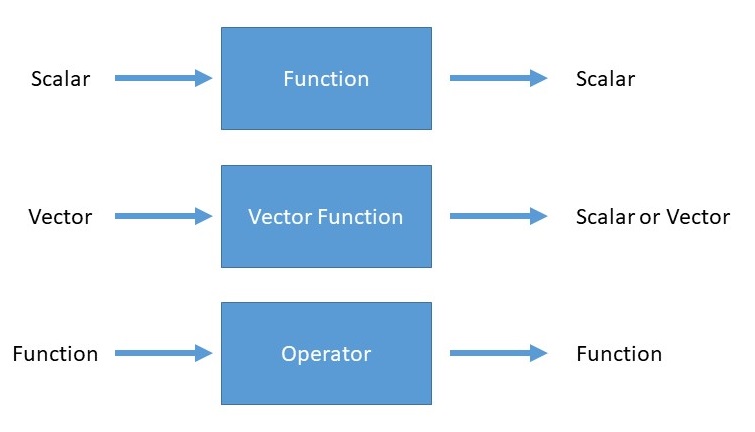
For the time-independent Schrödinger Equation, the operator of relevance is the Hamiltonian operator (often just called the Hamiltonian) and is the most ubiquitous operator in quantum mechanics.

$$\hat{H} = -\dfrac{\hbar^2}{2m}\nabla^2+V(\vec{r})$$

We often (but not always) indicate that an object is an operator by placing a `hat' over it, e.g., $\hat{H}$. So the time-independent Schrödinger Equation (Equation $\ref{3.1.19}$) can then be simplified to

$$\hat{H} \psi(\vec{r}) = E\psi(\vec{r}) \label{simple}$$

Equation $\ref{simple}$ says that the Hamiltonian operator operates on the wavefunction to produce the total energy, which is a number (i.e., a quantity or observable) times the wavefunction.

Fundamental Properties of Operators

Most properties of operators are straightforward, but they are summarized below for completeness.

The sum and difference of two operators $\hat{A}$ and $\hat{B}$ are given by

$$(\hat{A} \pm \hat{B}) f = \displaystyle \hat{A} f \pm \hat{B} f$$

The product of two operators is defined by

$$\hat{A} \hat{B} f \equiv \hat{A} [ \hat{B} f ]$$

Two operators are equal if

$$\hat{A} f = \hat{B} f$$

for all functions $f$.

The identity operator $\hat{1}$ does nothing (or multiplies by 1)

$${\hat 1} f = f$$

The associative law holds for operators

$$\hat{A}(\hat{B}\hat{C}) = (\hat{A}\hat{B})\hat{C}$$

The commutative law does not generally hold for operators. In general,

$$\hat{A} \hat{B} \neq \hat{B}\hat{A}$$

It is convenient to define the commutator of $\hat{A}$ and $\hat{B}$

$$[\hat{A}, \hat{B}] \equiv \hat{A} \hat{B} - \hat{B} \hat{A}$$

Note that the order matters, so that

$$[\hat{A} ,\hat{B} ] = - [\hat{B} ,\hat{A} ] .$$

If $\hat{A}$ and $\hat{B}$ commute, then

$$[\hat{A} ,\hat{B} ] = 0.$$

The $n$-th power of an operator $\hat{A}^n$ is defined as $n$ successive applications of the operator, e.g.

$$\hat{A}^2 f = \hat{A} \hat{A} f$$