
1: The Rise of Quantum Mechanics (Lecture)
- Page ID
- 198566
\( \newcommand{\vecs}[1]{\overset { \scriptstyle \rightharpoonup} {\mathbf{#1}} } \)
\( \newcommand{\vecd}[1]{\overset{-\!-\!\rightharpoonup}{\vphantom{a}\smash {#1}}} \)
\( \newcommand{\id}{\mathrm{id}}\) \( \newcommand{\Span}{\mathrm{span}}\)
( \newcommand{\kernel}{\mathrm{null}\,}\) \( \newcommand{\range}{\mathrm{range}\,}\)
\( \newcommand{\RealPart}{\mathrm{Re}}\) \( \newcommand{\ImaginaryPart}{\mathrm{Im}}\)
\( \newcommand{\Argument}{\mathrm{Arg}}\) \( \newcommand{\norm}[1]{\| #1 \|}\)
\( \newcommand{\inner}[2]{\langle #1, #2 \rangle}\)
\( \newcommand{\Span}{\mathrm{span}}\)
\( \newcommand{\id}{\mathrm{id}}\)
\( \newcommand{\Span}{\mathrm{span}}\)
\( \newcommand{\kernel}{\mathrm{null}\,}\)
\( \newcommand{\range}{\mathrm{range}\,}\)
\( \newcommand{\RealPart}{\mathrm{Re}}\)
\( \newcommand{\ImaginaryPart}{\mathrm{Im}}\)
\( \newcommand{\Argument}{\mathrm{Arg}}\)
\( \newcommand{\norm}[1]{\| #1 \|}\)
\( \newcommand{\inner}[2]{\langle #1, #2 \rangle}\)
\( \newcommand{\Span}{\mathrm{span}}\) \( \newcommand{\AA}{\unicode[.8,0]{x212B}}\)
\( \newcommand{\vectorA}[1]{\vec{#1}} % arrow\)
\( \newcommand{\vectorAt}[1]{\vec{\text{#1}}} % arrow\)
\( \newcommand{\vectorB}[1]{\overset { \scriptstyle \rightharpoonup} {\mathbf{#1}} } \)
\( \newcommand{\vectorC}[1]{\textbf{#1}} \)
\( \newcommand{\vectorD}[1]{\overrightarrow{#1}} \)
\( \newcommand{\vectorDt}[1]{\overrightarrow{\text{#1}}} \)
\( \newcommand{\vectE}[1]{\overset{-\!-\!\rightharpoonup}{\vphantom{a}\smash{\mathbf {#1}}}} \)
\( \newcommand{\vecs}[1]{\overset { \scriptstyle \rightharpoonup} {\mathbf{#1}} } \)
\( \newcommand{\vecd}[1]{\overset{-\!-\!\rightharpoonup}{\vphantom{a}\smash {#1}}} \)
\(\newcommand{\avec}{\mathbf a}\) \(\newcommand{\bvec}{\mathbf b}\) \(\newcommand{\cvec}{\mathbf c}\) \(\newcommand{\dvec}{\mathbf d}\) \(\newcommand{\dtil}{\widetilde{\mathbf d}}\) \(\newcommand{\evec}{\mathbf e}\) \(\newcommand{\fvec}{\mathbf f}\) \(\newcommand{\nvec}{\mathbf n}\) \(\newcommand{\pvec}{\mathbf p}\) \(\newcommand{\qvec}{\mathbf q}\) \(\newcommand{\svec}{\mathbf s}\) \(\newcommand{\tvec}{\mathbf t}\) \(\newcommand{\uvec}{\mathbf u}\) \(\newcommand{\vvec}{\mathbf v}\) \(\newcommand{\wvec}{\mathbf w}\) \(\newcommand{\xvec}{\mathbf x}\) \(\newcommand{\yvec}{\mathbf y}\) \(\newcommand{\zvec}{\mathbf z}\) \(\newcommand{\rvec}{\mathbf r}\) \(\newcommand{\mvec}{\mathbf m}\) \(\newcommand{\zerovec}{\mathbf 0}\) \(\newcommand{\onevec}{\mathbf 1}\) \(\newcommand{\real}{\mathbb R}\) \(\newcommand{\twovec}[2]{\left[\begin{array}{r}#1 \\ #2 \end{array}\right]}\) \(\newcommand{\ctwovec}[2]{\left[\begin{array}{c}#1 \\ #2 \end{array}\right]}\) \(\newcommand{\threevec}[3]{\left[\begin{array}{r}#1 \\ #2 \\ #3 \end{array}\right]}\) \(\newcommand{\cthreevec}[3]{\left[\begin{array}{c}#1 \\ #2 \\ #3 \end{array}\right]}\) \(\newcommand{\fourvec}[4]{\left[\begin{array}{r}#1 \\ #2 \\ #3 \\ #4 \end{array}\right]}\) \(\newcommand{\cfourvec}[4]{\left[\begin{array}{c}#1 \\ #2 \\ #3 \\ #4 \end{array}\right]}\) \(\newcommand{\fivevec}[5]{\left[\begin{array}{r}#1 \\ #2 \\ #3 \\ #4 \\ #5 \\ \end{array}\right]}\) \(\newcommand{\cfivevec}[5]{\left[\begin{array}{c}#1 \\ #2 \\ #3 \\ #4 \\ #5 \\ \end{array}\right]}\) \(\newcommand{\mattwo}[4]{\left[\begin{array}{rr}#1 \amp #2 \\ #3 \amp #4 \\ \end{array}\right]}\) \(\newcommand{\laspan}[1]{\text{Span}\{#1\}}\) \(\newcommand{\bcal}{\cal B}\) \(\newcommand{\ccal}{\cal C}\) \(\newcommand{\scal}{\cal S}\) \(\newcommand{\wcal}{\cal W}\) \(\newcommand{\ecal}{\cal E}\) \(\newcommand{\coords}[2]{\left\{#1\right\}_{#2}}\) \(\newcommand{\gray}[1]{\color{gray}{#1}}\) \(\newcommand{\lgray}[1]{\color{lightgray}{#1}}\) \(\newcommand{\rank}{\operatorname{rank}}\) \(\newcommand{\row}{\text{Row}}\) \(\newcommand{\col}{\text{Col}}\) \(\renewcommand{\row}{\text{Row}}\) \(\newcommand{\nul}{\text{Nul}}\) \(\newcommand{\var}{\text{Var}}\) \(\newcommand{\corr}{\text{corr}}\) \(\newcommand{\len}[1]{\left|#1\right|}\) \(\newcommand{\bbar}{\overline{\bvec}}\) \(\newcommand{\bhat}{\widehat{\bvec}}\) \(\newcommand{\bperp}{\bvec^\perp}\) \(\newcommand{\xhat}{\widehat{\xvec}}\) \(\newcommand{\vhat}{\widehat{\vvec}}\) \(\newcommand{\uhat}{\widehat{\uvec}}\) \(\newcommand{\what}{\widehat{\wvec}}\) \(\newcommand{\Sighat}{\widehat{\Sigma}}\) \(\newcommand{\lt}{<}\) \(\newcommand{\gt}{>}\) \(\newcommand{\amp}{&}\) \(\definecolor{fillinmathshade}{gray}{0.9}\)The traditional introduction to quantum mechanics involves discussing the breakdown of classical mechanics and where quantum steps in. We have three examples of this: (1) blackbody radiation, (2) photoelectric effect and (3) hydrogen emission (of light). We discuss them here.
First Evidence of Classical Breakdown: Blackbody Radiation
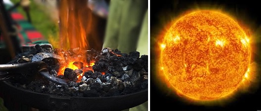
It has been known for a long time that hot things radiate light!
Blackbody Radiators
To begin analyzing heat radiation, we need to be specific about the body doing the radiating: the simplest possible case is an idealized body which is a perfect absorber, and therefore also (from the above argument) a perfect emitter. For obvious reasons, this is called a “blackbody”. It is an idealized physical body that absorbs all incident electromagnetic radiation, regardless of frequency or angle of incidence.
A blackbody radiator is an object or system that absorbs all radiation incident upon it and re-radiates energy which is characteristic of only the radiating system only, not on the type of radiation which is incident upon it.
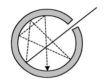
A physical realization of a blackbody is a cavity with a small hole with many reflections and absorptions. Very few entering photons (light rays) will get out. The inside of the cavity has radiation which is homogeneous and isotropic (the same in any direction, uniform everywhere).
Two experimental "laws" connected to black-body radiation:
- Stefan-Boltzmann Law: The total (i.e., integrated) radiation intensity varies as \(T^4\)
- Wien’s Displacement Law: As the temperature of a blackbody varies, so does the frequency at which the emitted radiation is most intense. In fact, that frequency is directly proportional to the absolute temperature:
\[\nu_{max} \propto T \label{-1}\]
where the proportionality constant is \(5.879 \times 10^{10} Hz/K\).
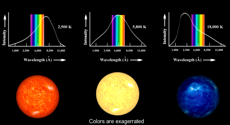
The concept underlying Equation \(\ref{-1}\) is familiar to most people. When an iron is heated in a fire, the first visible radiation (at around 900 K) is deep red, the lowest frequency visible light. Further increase in T causes the color to change to orange then yellow, and finally blue at very high temperatures (10,000 K or more) for which the peak in radiation intensity has moved beyond the visible into the ultraviolet (Figure \(\PageIndex{3}\)).
Classic Blackbody Radiation
Lord Rayleigh and J. H. Jeans developed an equation which explained blackbody radiation at low frequencies.The equation which seemed to express blackbody radiation was built upon all the known assumptions of physics at the time.
The big assumption which Rayleigh and Jean implied was that infinitesimal amounts of energy were continuously added to the system when the frequency was increased.
Classical physics assumed that energy emitted by atomic oscillations could have any continuous value.This was true for anything that had been studied up until that point, including things like acceleration, position, or energy. The resulting Rayleigh-Jeans law was
\[ d\rho \left( \nu ,T \right) = \rho_{\nu}\left( T \right) d\nu = \underbrace{\dfrac{8 \pi k_B T}{c^3} \nu^2}_{\text{Rayleigh-Jeans distribution}} d\nu \label{0}\]
The Classical Rayleigh-Jeans law
Assumed that energy emitted by atomic oscillations could have any continuous value.
Aside: Distributions
Equation \(\ref{0}\) is a "distribution" not unlike the distribution of grades in a course. As such it has several properties of interest:
- The integrated value (\(A\)): This is the sum over the distribution over all possible values of \(x\). Graphically, this is the area under the distribution. \[ A= \int_{-\infty}^{\infty} D(x)\, dx \label{1}\] If the range of \(x\) is less than \(-\infty\) to \(\infty\) (e.g., from \(a\) to \(b)\), then \(A\) is given by \[ A = \int_{a}^{b} D(x)\, dx \label{2}\]
- The expectation value (\(\langle x \rangle \)): This is a different term that is used synonymously with the average (or mean) of \(x\) over the distribution. The mean is given by \[ \bar{x} = \langle x \rangle = \int_{a}^{b} x D(x)\, dx \label{3}\] Notice the difference between Equations \(\ref{2}\) and \(\ref{3}\).
- The most probable value (\(x_{mp}\)): This is the value of \(x\) at the peak of \(D(x)\). This is determined from basic calculus for determining extrema and via identifying when the derivative of the distribution is zero. \[ \left( \dfrac{dD(x)}{dx} \right)_{x_{mp}} = 0 \label{4}\]
- The standard deviation (\(\sigma_x\)): This is the a measure of the spread of the distribution and is given by \[ \sigma_x^2 = \int_{a}^{b} (x-\bar{x})^2 D(x) \,dx \label{5}\]
Experimental data performed on the black box showed slightly different results than what was expected by the Rayleigh-Jeans law. The law had been studied and widely accepted by many physicists of the day, but the experimental results did not lie, something was different between what was theorized and what actually happens.The experimental results showed a bell type of curve but according to the Rayleigh-Jeans law the frequency diverged as it neared the ultraviolet region (Equation \(\ref{0}\)). This inconsistency was termed the ultraviolet catastrophe.
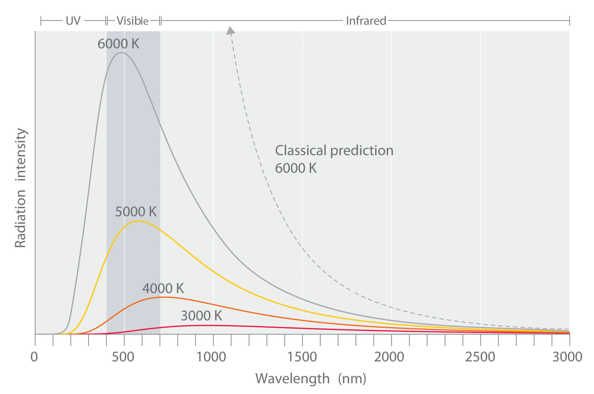
Max Planck was the first person to properly explain this experimental data. Rayleigh and Jean made the assumption that energy is continuous, but Planck took a slightly different approach. He said energy must come in certain unit intervals instead of being any random unit or number. He instead “quantized” energy in the form of
\[E= nh\nu\]
where \(n\) is an integer, \(h\) is a constant, and \(\nu\) is the frequency. This assumption proved to be the missing piece of the puzzle and Planck derived an expression which could explain the experimental data.
Max Planck proposed that energy is emitted in discrete packets - he didn't know what they were though.
From this, the Planck distribution law, with respect to frequency, was derived from
\[d\rho(\nu,T) = \rho_\nu (T) d\nu = \underbrace{\dfrac {2 h}{c^3} \cdot \dfrac {\nu^3 }{e^{\frac {h\nu}{k_B T}}-1}}_{\text{Planck's distribution}} d\nu \label{Planck1}\]
which is the "radiant energy density function".
using:
- \(\pi\) = 3.14159
- \(h\) = \(6.626 \times 10^{-34} J\cdot s\)
- \(c\) = \(3.00 \times 10^{8} \dfrac {M}{s}\)
- \(v\) = \(\dfrac {1}{s}\)
- \(k_B\) = \(1.38 \times 10^{-23} \dfrac {J}{K}\)
- \(T\) is absolute temperature (in Kelvin)
The resulting units of the radiant energy density function can be shown to be \(J \cdot m^{-3}\) by using the constants and their respective units.
By setting the wavelength \(\lambda\) = \(c \cdot \nu^{-1}\) and \(d\nu\) = \(c \cdot \dfrac {-d\lambda}{\lambda^2}\), you can express \(d\rho\) (\ref{Planck1}) in terms of \(\lambda\) rather than \(\nu\).
\[d\rho (\lambda, T) = \rho_\lambda (T)d\lambda = \underbrace{\dfrac {2 hc^2}{\lambda^5} \cdot \dfrac {1}{e^{\frac {hc}{\lambda k_B T}}-1} }_{\text{Planck's distribution}} d\lambda\label{Planck2}\]
Both the Stefan-Boltzmann Law and the Wien’s Displacement Law can be derived from Planck's distribution.
Example \(\PageIndex{1}\): Peak Wavelength
The maximum of a curve has slope equal to zero, so to find \(\lambda_{max}\), set
\[\dfrac {d\rho_\lambda (T)}{d\lambda} = 0\]
which results in
\[\lambda_{max} = \dfrac {hc}{4.965k_B T} \label{10}\]
From this Equation \(\ref{10}\), it is clear that temperature and the maximum wavelength are inversely proportional. A larger temperature gives a smaller \(\lambda_{max}\), where a smaller temperature gives a larger \(\lambda_{max}\).
Interactive: Blackbody Spectrum
The mathematics implied that the energy given off by a blackbody was not continuous, but given off at certain specific wavelengths, in regular increments. If Planck assumed that the energy of blackbody radiation was in the form
\[E = nh \nu\]
where \(n\) is an integer (now called a quantum number), then he could explain what the mathematics represented.
Continued in Lecture 2: The Rise of Quantum Mechanics