3.6: Interaction Picture

The interaction picture is a hybrid representation that is useful in solving problems with time-dependent Hamiltonians in which we can partition the Hamiltonian as

\[H (t) = H_0 + V (t) \label{2.93}\]

\(H_0\) is a Hamiltonian for the degrees of freedom we are interested in, which we treat exactly, and can be (although for us usually will not be) a function of time. \(V(t)\) is a time-dependent potential which can be complicated. In the interaction picture, we will treat each part of the Hamiltonian in a different representation. We will use the eigenstates of \(H_0\) as a basis set to describe the dynamics induced by \(V(t)\), assuming that \(V(t)\) is small enough that eigenstates of \(H_0\) are a useful basis. If \(H_0\) is not a function of time, then there is a simple time-dependence to this part of the Hamiltonian that we may be able to account for easily. Setting \(V\) to zero, we can see that the time evolution of the exact part of the Hamiltonian \(H_0\) is described by

\[\frac {\partial} {\partial t} U_0 \left( t , t_0 \right) = - \frac {i} {\hbar} H_0 (t) U_0 \left( t , t_0 \right) \label{2.94}\]

where,

\[U_0 \left( t , t_0 \right) = \exp _ {+} \left[ - \frac {i} {\hbar} \int _ {t_0}^{t} d \tau H_0 (t) \right] \label{2.95}\]

or, for a time-independent \(H_0\),

\[U_0 \left( t , t_0 \right) = e^{- i H_0 \left( t - t_0 \right) / \hbar} \label{2.96}\]

We define a wavefunction in the interaction picture \(| \psi _ {I} \rangle\) in terms of the Schrödinger wavefunction through:

\[| \psi _ {S} (t) \rangle \equiv U_0 \left( t , t_0 \right) | \psi _ {I} (t) \rangle \label{2.97}\]

or

\[| \psi _ {I} \rangle = U_0^{\dagger} | \psi _ {S} \rangle \label{2.98}\]

Effectively the interaction representation defines wavefunctions in such a way that the phase accumulated under \(e^{- i H_0 t / h}\) is removed. For small \(V\), these are typically high frequency oscillations relative to the slower amplitude changes induced by \(V\).

Now we need an equation of motion that describes the time evolution of the interaction picture wavefunctions. We begin by substituting Equation \ref{2.97} into the TDSE:

\[ \begin{align} | \psi _ {S} (t) \rangle & = U_0 \left( t , t_0 \right) | \psi _ {1} (t) \rangle \\[4pt] & = U_0 \left( t , t_0 \right) U _ {I} \left( t , t_0 \right) | \psi _ {I} \left( t_0 \right) \rangle \\[4pt] & = U_0 \left( t , t_0 \right) U _ {I} \left( t , t_0 \right) | \psi _ {S} \left( t_0 \right) \rangle \\[4pt] \therefore \quad U & \left( t , t_0 \right) = U_0 \left( t , t_0 \right) U _ {I} \left( t , t_0 \right) \end{align} \]

\[\therefore \quad i \hbar \frac {\partial | \psi _ {I} \rangle} {\partial t} = V_I | \psi _ {I} \rangle \label{2.101}\]

where

\[V_I (t) = U_0^{\dagger} \left( t , t_0 \right) V (t) U_0 \left( t , t_0 \right) \label{2.102}\]

\(| \psi _ {I} \rangle\) satisfies the Schrödinger equation with a new Hamiltonian in Equation \ref{2.102}: the interaction picture Hamiltonian, \(V_I(t)\). We have performed a unitary transformation of \(V(t)\) into the frame of reference of \(H_0\), using \(U_0\). Note: Matrix elements in

\[V_I = \left\langle k \left| V_I \right| l \right\rangle = e^{- i \omega _ {l k} t} V _ {k l}\]

where \(k\) and \(l\) are eigenstates of \(H_0\). We can now define a time-evolution operator in the interaction picture:

\[| \psi _ {I} (t) \rangle = U _ {I} \left( t , t_0 \right) | \psi _ {I} \left( t_0 \right) \rangle \label{2.103}\]

where

\[U _ {I} \left( t , t_0 \right) = \exp _ {+} \left[ \frac {- i} {\hbar} \int _ {t_0}^{t} d \tau V_I ( \tau ) \right] \label{2.104}\]

Now we see that

\[\begin{aligned}
\left|\psi_{S}(t)\right\rangle &=U_{0}\left(t, t_{0}\right)\left|\psi_{I}(t)\right\rangle \\[4pt]
&=U_{0}\left(t, t_{0}\right) U_{I}\left(t, t_{0}\right)\left|\psi_{I}\left(t_{0}\right)\right\rangle \\[4pt]
&=U_{0}\left(t, t_{0}\right) U_{I}\left(t, t_{0}\right)\left|\psi_{S}\left(t_{0}\right)\right\rangle
\end{aligned}\]

\[\therefore U\left(t, t_{0}\right)=U_{0}\left(t, t_{0}\right) U_{I}\left(t, t_{0}\right)\label{2.106}\]

Also, the time evolution of conjugate wavefunction in the interaction picture can be written

\[U^{\dagger} \left( t , t_0 \right) = U _ {I}^{\dagger} \left( t , t_0 \right) U_0^{\dagger} \left( t , t_0 \right) = \exp _ {-} \left[ \frac {i} {\hbar} \int _ {t_0}^{t} d \tau V_I ( \tau ) \right] \exp _ {-} \left[ \frac {i} {\hbar} \int _ {t_0}^{t} d \tau H_0 ( \tau ) \right] \label{2.107}\]

For the last two expressions, the order of these operators certainly matters. So what changes about the time-propagation in the interaction representation? Let’s start by writing out the time-ordered exponential for \(U\) in Equation \ref{2.106} using Equation \ref{2.104}:

\[ \begin{align} U \left( t , t_0 \right) &= U_0 \left( t , t_0 \right) + \left( \frac {- i} {\hbar} \right) \int _ {t_0}^{t} d \tau U_0 ( t , \tau ) V ( \tau ) U_0 \left( \tau , t_0 \right) + \cdots \\[4pt] &= U_0 \left( t , t_0 \right) + \sum _ {n = 1}^{\infty} \left( \frac {- i} {\hbar} \right)^{n} \int _ {t_0}^{t} d \tau _ {n} \int _ {t_0}^{\tau _ {n}} d \tau _ {n - 1} \cdots \int _ {t_0}^{\tau _ {2}} d \tau _ {1} U_0 \left( t , \tau _ {n} \right) V \left( \tau _ {n} \right) U_0 \left( \tau _ {n} , \tau _ {n - 1} \right) \ldots \times U_0 \left( \tau _ {2} , \tau _ {1} \right) V \left( \tau _ {1} \right) U_0 \left( \tau _ {1} , t_0 \right) \label{2.108} \end{align}\]

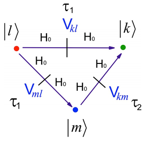
Here I have used the composition property of \(U \left( t , t_0 \right)\). The same positive time-ordering applies. Note that the interactions \(V(\tau_i)\) are not in the interaction representation here. Rather we used the definition in Equation \ref{2.102} and collected terms. Now consider how \(U\) describes the timedependence if \(I\) initiate the system in an eigenstate of \(H_0\), \(| l \rangle\) and observe the amplitude in a target eigenstate \(| k \rangle\). The system evolves in eigenstates of \(H_0\) during the different time periods, with the time-dependent interactions \(V\) driving the transitions between these states. The first-order term describes direct transitions between \(l\) and \(k\) induced by \(V\), integrated over the full time period. Before the interaction phase is acquired as \(e^{- i E _ {\ell} \left( \tau - t_0 \right) / \hbar}\), whereas after the interaction phase is acquired as \(e^{- i E _ {\ell} ( t - \tau ) / \hbar}\). Higher-order terms in the time-ordered exponential accounts for all possible intermediate pathways.

We now know how the interaction picture wavefunctions evolve in time. What about the operators? First of all, from examining the expectation value of an operator we see

\[\left.\begin{aligned} \langle \hat {A} (t) \rangle & = \langle \psi (t) | \hat {A} | \psi (t) \rangle \\[4pt] & = \left\langle \psi \left( t_0 \right) \left| U^{\dagger} \left( t , t_0 \right) \hat {A} U \left( t , t_0 \right) \right| \psi \left( t_0 \right) \right\rangle \\[4pt] & = \left\langle \psi \left( t_0 \right) \left| U _ {I}^{\dagger} U_0^{\dagger} \hat {A} U_0 U _ {I} \right| \psi \left( t_0 \right) \right\rangle \\[4pt] & = \left\langle \psi _ {L} (t) \left| \hat {A} _ {L} \right| \psi _ {L} (t) \right\rangle \end{aligned} \right. \label{2.109}\]

where

\[A _ {I} \equiv U_0^{\dagger} A _ {S} U_0 \label{2.110}\]

So the operators in the interaction picture also evolve in time, but under \(H_0\). This can be expressed as a Heisenberg equation by differentiating

\[\frac {\partial} {\partial t} \hat {A} _ {I} = \frac {i} {\hbar} \left[ H_0 , \hat {A} _ {I} \right] \label{2.111}\]

Also, we know

\[\frac {\partial} {\partial t} | \psi _ {I} \rangle = \frac {- i} {\hbar} V_I (t) | \psi _ {I} \rangle \label{2.112}\]

Notice that the interaction representation is a partition between the Schrödinger and Heisenberg representations. Wavefunctions evolve under VI , while operators evolve under

\[\text {For} H_0 = 0 , V (t) = H \quad \Rightarrow \quad \frac {\partial \hat {A}} {\partial t} = 0 ; \quad \frac {\partial} {\partial t} | \psi _ {S} \rangle = \frac {- i} {\hbar} H | \psi _ {S} \rangle \text{For Schrödinger} \]

\[\text {For} H_0 = H , V (t) = 0 \Rightarrow \frac {\partial \hat {A}} {\partial t} = \frac {i} {\hbar} [ H , \hat {A} ] ; \quad \frac {\partial \psi} {\partial t} = 0 \text{For Heisenberg} \label{2.113}\]

The relationship between UI and bn

Earlier we described how time-dependent problems with Hamiltonians of the form \(H = H_0 + V (t)\) could be solved in terms of the time-evolving amplitudes in the eigenstates of \(H_0\). We can describe the state of the system as a superposition

\[| \psi (t) \rangle = \sum _ {n} c _ {n} (t) | n \rangle \label{2.114}\]

where the expansion coefficients \(c _ {k} (t)\) are given by

\[\left.\begin{aligned} c _ {k} (t) & = \langle k | \psi (t) \rangle = \left\langle k \left| U \left( t , t_0 \right) \right| \psi \left( t_0 \right) \right\rangle \\[4pt] & = \left\langle k \left| U_0 U _ {I} \right| \psi \left( t_0 \right) \right\rangle \\[4pt] & = e^{- i E _ {k} t / \hbar} \left\langle k \left| U _ {I} \right| \psi \left( t_0 \right) \right\rangle \end{aligned} \right. \label{2.115}\]

Now, comparing equations \ref{2.115} and \ref{2.54} allows us to recognize that our earlier modified expansion coefficients \(b_n\) were expansion coefficients for interaction picture wavefunctions

\[b _ {k} (t) = \langle k | \psi _ {I} (t) \rangle = \left\langle k \left| U _ {I} \right| \psi \left( t_0 \right) \right\rangle \label{2.116}\]

Readings

1. Mukamel, S., Principles of Nonlinear Optical Spectroscopy. Oxford University Press: New York, 1995.
2. Nitzan, A., Chemical Dynamics in Condensed Phases. Oxford University Press: New York, 2006; Ch. 4.