1.1: Markov Processes

Probability Distributions and Transitions

Suppose that an arbitrary system of interest can be in any one of \(N\) distinct states. The system could be a protein exploring different conformational states; or a pair of molecules oscillating between a "reactants" state and a "products" state; or any system that can sample different states over time. Note here that \(N\) is finite, that is, the available states are discretized. In general, we could consider systems with a continuous set of available states (and we will do so in section 1.3), but for now we will confine ourselves to the case of a finite number of available states. In keeping with our discretization scheme, we will also (again, for now) consider the time evolution of the system in terms of discrete timesteps rather than a continuous time variable.

Let the system be in some unknown state \(m\) at timestep \(s\), and suppose we’re interested in the probability of finding the system in a specific state \(n\), possibly but not necessarily the same as state \(m\), at the next timestep \(s+1\). We will denote this probability by

\[P(n, s+1)\]

If we had knowledge of \(m\), then this probability could be described as the probability of the system being in state \(n\) at timestep \(s+1\) given that the system was in state \(m\) at timestep \(s\). Probabilities of this form are known as conditional probabilities, and we will denote this conditional probability by

\[Q(m, s \mid n, s+1)\]

In many situations of physical interest, the probability of a transition from state \(m\) to state \(n\) is time-independent, depending only on the nature of \(m\) and \(n\), and so we drop the timestep arguments to simplify the notation,

\[Q(m, s \mid n, s+1) \equiv Q(m, n)\]

This observation may seem contradictory, because we are interested in the time-dependent probability of observing a system in a state \(n\) while also claiming that the transition probability described above is time-independent. But there is no contradiction here, because the transition probability \(Q\) - a conditional probability - is a different quantity from the time-dependent probability \(P\) we are interested in. In fact, we can express \(P(n, s+1)\) in terms of \(Q(m, n)\) and other quantities as follows:

Since we don’t know the current state \(m\) of the system, we consider all possible states \(m\) and multiply the probability that the system is in state \(m\) at timestep \(s\) by the probability of the system being in state \(n\) at timestep \(s+1\) given that it is in state \(m\) at timestep \(s\). Summing over all possible states \(m\) gives \(P\left(n, s_{1}\right)\) at timestep \(s+1\) in terms of the corresponding probabilities at timestep \(s\).

Mathematically, this formulation reads

\[P(n, s+1)=\sum_{m} P(m, s) Q(m, n)\]

We’ve made some progress towards a practical method of finding \(P(n, s+1)\), but the current formulation Eq.(1.1) requires knowledge of both the transition probabilities \(Q(m, n)\) and the probabilities \(P(m, s)\) for all states \(m\). Unfortunately, \(P(m, s)\) is just as much a mystery to us as \(P(n, s+1)\). What we usually know and control in experiments are the initial conditions; that is, if we prepare the system in state \(k\) at timestep \(s=0\), then we know that \(P(k, 0)=1\) and \(P(n, 0)=0\) for all \(n \neq k\). So how do we express \(P(n, s+1)\) in terms of the initial conditions of the experiment?

We can proceed inductively: if we can write \(P(n, s+1)\) in terms of \(P(m, s)\), then we can also write \(P(m, s)\) in terms of \(P(l, s-1)\) by the same approach:

\[P(n, s+1)=\sum_{l, m} P(l, s-1) Q(l, m) Q(m, n)\]

Note that \(Q\) has two parameters, each of which can take on \(N\) possible values. Consequently we may choose to write \(Q\) as an \(N \times N\) matrix \(\mathbf{Q}\) with matrix elements \((\mathbf{Q})_{m n}=Q(m, n)\). Rearranging the sums in Eq.(1.2) in the following manner,

\[P(n, s+1)=\sum_{l} P(l, s-1) \sum_{m} Q(l, m) Q(m, n)\]

we recognize the sum over \(m\) as the definition of a matrix product,

\[\sum_{m}(\mathbf{Q})_{l m}(\mathbf{Q})_{m n}=\left(\mathbf{Q}^{2}\right)_{l n}\]

Hence, Eq.(1.2) can be recast as

\[P(n, s+1)=\sum_{l} P(l, s-1)\left(\mathbf{Q}^{2}\right)_{l n}\]

This process can be continued inductively until \(P(n, s+1)\) is written fully in terms of initial conditions. The final result is:

\[\begin{aligned} P(n, s+1) &=\sum_{m} P(m, 0)\left(\mathbf{Q}^{s+1}\right)_{m n} \\ &=P(k, 0)\left(\mathbf{Q}^{s+1}\right)_{m n} \end{aligned}\]

where \(k\) is the known initial state of the system (all other \(m\) do not contribute to the sum since \(P(m, 0)=0\) for \(m \neq k\) ). Any process that can be described in this manner is called a Markov process, and the sequence of events comprising the process is called a Markov chain.

A more rigorous discussion of the origins and nature of Markov processes may be found in, e.g., de Groot and Mazur [2].

The Transition Probability Matrix

We now consider some important properties of the transition probability matrix \(\mathbf{Q}\). By virtue of its definition, \(Q\) is not necessarily Hermitian: if it were Hermitian, every conceivable transition between states would have to have the same forward and backward probability, which is often not the case.

Example: Consider a chemical system that can exist in either a reactant state A or a product state B, with forward reaction probability \(p\) and backward reaction probability \(q=1-p\),

\[\mathrm{A} \underset{q}{\stackrel{p}{\rightleftharpoons}} \mathrm{B}\]

The transition probability matrix \(\mathbf{Q}\) for this system is the \(2 \times 2\) matrix

\[\mathbf{Q}=\left(\begin{array}{ll} q & p \\ q & p \end{array}\right)\]

To construct this matrix, we first observe that the given probabilities directly describe the off-diagonal elements \(Q_{A B}\) and \(Q_{B A}\); then we invoke conservation of probability. For example, if the system is in the reactant state \(A\), it can only stay in \(A\) or react to form product \(B\); there are no other possible outcomes, so we must have \(Q_{A A}+Q_{A B}=1 .\) This forces the value \(1-p=q\) upon \(Q_{A A}\), and a similar argument yields \(Q_{B B}\).

Clearly this matrix is not symmetric, hence it is not Hermitian either, thus demonstrating our first general observation about \(\mathbf{Q}\).

The non-Hermiticity of \(\mathbf{Q}\) implies also that its eigenvalues \(\lambda_{i}\) are not necessarily real-valued. Nevertheless, \(\mathbf{Q}\) yields two sets of eigenvectors, a left set \(\chi_{i}\) and a right set \(\phi_{i}\), which satisfy the relations

\[\begin{aligned} &\chi_{i} \mathbf{Q}=\lambda_{i} \chi_{i} \\ &\mathbf{Q} \phi_{i}=\lambda_{i} \phi_{i} \end{aligned}\]

The left- and right-eigenvectors of \(\mathbf{Q}\) are orthonormal,

\[\left\langle\chi_{i} \mid \phi_{j}\right\rangle=\delta_{i j}\]

and they form a complete set, hence there is a resolution of the identity of the form

\[\sum_{i}\left|\phi_{i}\right\rangle\left\langle\chi_{i}\right|=1\]

Conservation of probability further restricts the elements of \(\mathbf{Q}\) to be nonnegative with \(\sum_{n} \mathbf{Q}_{m n}=1\). It can be shown that this condition guarantees that all eigenvalues of \(\mathbf{Q}\) are bounded by the unit circle in the complex plane,

\[\left|\lambda_{i}\right| \leq 1, \forall i\]

Proof of Eq. (1.12): The \(i^{\text {th }}\) eigenvalue of \(\mathrm{Q}\) satisfies

\[\lambda_{i} \phi_{i}(n)=\sum_{m} Q_{n m} \phi_{i}(m)\]

for each \(n\). Take the absolute value of this relation,

\[\left|\lambda_{i} \phi_{i}(n)\right|=\left|\sum_{m} Q_{n m} \phi_{i}(m)\right|\]

Now we can apply the triangle inequality to the right hand side of the equation:

\[\left|\sum_{m} Q_{n m} \phi_{i}(m)\right| \leq \sum_{m}\left|Q_{n m} \phi_{i}(m)\right|\]

Also, since all elements of \(\mathbf{Q}\) are nonnegative,

\[\left|\lambda_{i} \phi_{i}(n)\right| \leq \sum_{m} Q_{n m}\left|\phi_{i}(m)\right|\]

Now, the \(\phi_{i}(n)\) are finite, so there must be some constant \(c\) such that

\[\left|\phi_{i}(n)\right| \leq c\]

for all \(n\). Then our triangle inequality relation reads

\[c\left|\lambda_{i}\right| \leq c \sum_{m} Q_{n m}\]

Finally, since \(\sum_{m} Q_{n m}=1\), we have the desired result,

\[\left|\lambda_{i}\right| \leq 1\]

Another key feature of the transition probability matrix \(\mathbf{Q}\) is the following claim, which is intimately connected with the notion of an equilibrium state:

\[\text { Q always has the eigenvalue } \lambda=1\]

Proof of Eq.(1.13): We refer now to the left eigenvectors of \(\mathbf{Q}:\) a given left eigenvector \(\chi_{i}\) satisfies

\[\chi_{i}(n) \lambda_{i}=\sum_{m} \chi_{i}(m) Q_{m n}\]

Summing over \(n\), we find

\[\sum_{n} \chi_{i}(n) \lambda_{i}=\sum_{n} \sum_{m} \chi_{i}(m) Q_{m n}=\sum_{m} \chi_{i}(m)\]

since \(\sum_{m} Q_{n m}=1\). Thus, we have the following secular equation:

\[\left(\lambda_{i}-1\right) \sum_{n} \chi_{i}(n)=0\]

Clearly, \(\lambda=1\) is one of the eigenvalues satisfying this equation.

The decomposition of the secular equation in the preceding proof has a direct physical interpretation: the eigenvalue \(\lambda_{1}=1\) has a corresponding eigenvector which satisfies \(\sum_{n} \chi_{1}(n)=1\); this stationary-state eigensolution corresponds to the steady state of a system \(\chi_{1}(n)=P_{\mathrm{st}}(n)\). It then follows from the normalization condition that \(\phi_{1}(n)=1\). The remaining eigenvalues \(\left|\lambda_{j}\right|<1\) each satisfy \(\sum_{n} \chi_{j}(n)=0\) and hence correspond to zero-sum fluctuations about the equilibrium state.

In light of these properties of \(\mathbf{Q}\), we can define the time-dependent evolution of a system in terms of the eigenstates of \(\mathbf{Q}\); this representation is termed the spectral decomposition of \(P(n, s)\) (the set of eigenvalues of a matrix is also known as the spectrum of that matrix). In the basis of left and right eigenvectors of \(\mathbf{Q}\), the probability of being in state \(n\) at timestep \(s\), given the initial state as \(n_{0}\), is

\[P(n, s)=\left\langle n_{0}\left|\mathbf{Q}^{s}\right| n\right\rangle=\sum_{i}\left\langle n_{0} \mid \phi_{i}\right\rangle \lambda_{i}^{s}\left\langle\chi_{i} \mid n\right\rangle\]

If we (arbitrarily) assign the stationary state to \(i=1\), we have \(\lambda_{1}=1\) and \(\chi_{1}=P_{s t}\), where \(P_{s t}\) is the steady-state or equilibrium probability distribution. Thus,

\[P(n, s)=P_{s t}(n)+\sum_{i \neq 1} \phi_{i}\left(n_{0}\right) \lambda_{i}^{s} \chi_{i}(n)\]

The spectral decomposition proves to be quite useful in the analysis of more complicated probability distributions, especially those that have sufficiently many states as to require computational analysis.

Example: Consider a system which has three states with transition probabilities as illustrated in Figure 1.1. Notice that counterclockwise and clockwise transitions have differing probabilities, which allows this system to exhibit a net current or flux. Also, suppose that \(p+q=1\) so that the system must switch states at every timestep.

Figure 1.1: A simple three-state system with nonzero flux

The transition probability matrix for this system is

\[\mathbf{Q}=\left(\begin{array}{lll} 0 & p & q \\ q & 0 & p \\ p & q & 0 \end{array}\right)\]

To determine \(P(s)\), we find the eigenvalues and eigenvectors of this matrix and use the spectral decomposition, Eq.(1.14). The secular equation is

\[\operatorname{Det}(\mathbf{Q}-\lambda \mathbf{I})=\mathbf{0}\]

and its roots are

\[\lambda_{1}=1, \quad \lambda_{\pm}=-\frac{1}{2} \pm \frac{1}{2} \sqrt{3(4 p q-1)}\]

Notice that the nonequilibrium eigenvalues are complex unless \(p=q=\frac{1}{2}\), which corresponds to the case of vanishing net flux. If there is a net flux, these complex eigenvalues introduce an oscillatory behavior to \(P(s)\).

In the special case \(p=q=\frac{1}{2}\), the matrix \(\mathbf{Q}\) is symmetric, so the left and right eigenvectors are identical,

\[\begin{aligned} \chi_{1} &=\phi_{1}^{T}=\frac{1}{\sqrt{3}}(1,1,1) \\ \chi_{2} &=\phi_{2}^{T}=\frac{1}{\sqrt{6}}(1,1,-2) \\ \chi_{3} &=\phi_{3}^{T}=\frac{1}{\sqrt{2}}(1,-1,0) \end{aligned}\]

where \(T\) denotes transposition. Suppose the initial state is given as state 1 , and we’re interested in the probability of being in state 3 at timestep \(s, P_{1 \rightarrow 3}(s)\). According to the spectral decomposition formula \(\mathrm{Eq} \cdot(1.14)\)

\[\begin{aligned} P_{1 \rightarrow 3}(s)=& \sum_{i} \phi_{i}(1) \lambda_{i}^{s} \chi_{i}(3) \\ =&\left(\frac{1}{\sqrt{3}}\right)\left(1^{s}\right)\left(\frac{1}{\sqrt{3}}\right) \\ &+\left(\frac{1}{\sqrt{6}}\right)(1)\left(-\frac{1}{2}\right)^{s}\left(\frac{1}{\sqrt{6}}\right)(-2) \\ &+\left(\frac{1}{\sqrt{2}}\right)(1)\left(-\frac{1}{2}\right)^{s}\left(\frac{1}{\sqrt{2}}\right)(0) \\ P_{1 \rightarrow 3}(s)=& \frac{1}{3}-\frac{1}{3}\left(-\frac{1}{2}\right)^{s} \end{aligned}\]

Note that in the evaluation of each term, the first element of each left eigenvector \(\chi\) and the third element of each right eigenvector \(\phi\) was used, since we’re interested in the transition from state 1 to state 3 . Figure \(1.2\) is a plot of \(P_{1 \rightarrow 3}(s)\); it shows that the probability oscillates about the equilibrium value of \(\frac{1}{3}\), approaching the equilibrium value asymptotically.

Figure 1.2: Probability of a transition from state 1 to state 3 vs. number of timesteps. Black points correspond to actual timesteps; grey points have been interpolated to emphasize the oscillatory nature of \(P(s)\).

Detailed Balance

Our last topic of consideration within the subject of Markov processes is the notion of detailed balance, which is probably already somewhat familiar from elementary kinetics. Formally, a Markov process with transition probability matrix \(\mathbf{Q}\) satisfies detailed balance if the following condition holds:

\[P_{\mathrm{st}}(n) Q_{n m}=P_{\mathrm{st}}(m) Q_{m n}\]

And this steady state defines the equilibrium distribution:

\[P_{\mathrm{eq}}(n)=P_{\mathrm{st}}(n)=\lim _{t \rightarrow \infty} P(n, t)\]

This relation generalizes the notion of detailed balance from simple kinetics that the rates of forward and backward processes at equilibrium should be equal: here, instead of considering only a reactant state and a product state, we require that all pairs of states be related by Eq.(1.16).

Note also that this detailed balance condition is more general than merely requiring that \(\mathbf{Q}\) be symmetric, as the simpler definition from elementary kinetics would imply. However, if a system obeys detailed balance, we can describe it using a symmetric matrix via the following transformation: let

\[V_{n m}=\frac{\sqrt{P_{\mathrm{st}}(n)}}{\sqrt{P_{\mathrm{st}}(m)}} Q_{n m}\]

If we make the substitution \(P(n, s)=\sqrt{P_{\mathrm{st}}(n)} \cdot \tilde{P}(n, s)\), some manipulation using equations (1.1) and (1.17) yields

\[\frac{d \tilde{P}(n, t)}{d t}=\sum_{m} \tilde{P}(m, t) V_{m n}\]

The derivative \(\frac{d \tilde{P}(n, s)}{d t}\) here is really the finite difference \(\tilde{P}(n, s+1)-\tilde{P}(n, s)\) since we are considering discrete-time Markov processes, but we have introduced the derivative notation for comparison of this formula to later results for continuous-time systems.

As we did for \(\mathbf{Q}\), we can set up an eigensystem for \(\mathbf{V}\), which yields a spectral decomposition similar to that of \(\mathbf{Q}\) with the exception that the left and right eigenvectors \(\psi\) of \(\mathbf{V}\) are identical since \(\mathbf{V}\) is symmetric; in other words, \(\left\langle\psi_{i} \mid \psi_{j}\right\rangle=\delta_{i j}\). Furthermore, it can be shown that all eigenvalues not corresponding to the equilibrium state are either negative or zero; in particular, they are real. The eigenvectors of \(\mathbf{V}\) are related to the left and right eigenvectors of \(\mathbf{Q}\) by

\[\left|\phi_{i}\right\rangle=\frac{1}{\sqrt{P_{\mathrm{st}}}}\left|\psi_{i}\right\rangle \quad \text { and } \quad\left\langle\chi_{i}\right|=\sqrt{P_{\mathrm{st}}}\left\langle\psi_{i}\right|\]

Example: Our final model Markovian system is a linear three-state chain (Figure 1.3) in which the system must pass through the middle state in order to get from either end of the chain to the other. Again we require that \(p+q=1\). From this information, we can construct \(\mathbf{Q}\),

\[\mathbf{Q}=\left(\begin{array}{ccc} q & p & 0 \\ q & 0 & p \\ 0 & q & p \end{array}\right)\]

Notice how the difference between the three-site linear chain and the three-site ring of the previous example is manifest in the structure of \(\mathbf{Q}\), particularly in the direction of the zero diagonal. This structural difference carries through to general \(N\)-site chains and rings.

To determine the equilibrium probability distribution \(P_{\text {st }}\) for this system, one could multiply \(\mathbf{Q}\) by itself many times over and hope to find an analytic formula for \(\lim _{s \rightarrow \infty} \mathbf{Q}^{s} ;\) however, a less tedious and more intuitive approach is the following:

Noticing that the system cannot stay in state 2 at time \(s\) if it is already in state 2 at time \(s-1\), we conclude that \(P(1, s+2)\) depends only on \(P(1, s)\) and \(P(3, s)\). Also, the conditional probabilities \(P(1, s+2 \mid 1, s)\) and \(P(1, s+2 \mid 3, s)\) are both equal to \(q^{2}\). Likewise, \(P(3, s+2 \mid 1, s)\) and \(P(3, s+2 \mid 3, s)\) are both equal to \(p^{2} .\) Finally, if the system is in state 2 at time \(s\), it can only get back to state 2 at time \(s+2\) by passing through either state 1 or state 3 at time \(s+1\). The probability of either of these occurrences is \(p q\).

Figure 1.3: A three-state system in which sites are no longer identical

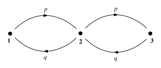
So the ratio \(P_{\mathrm{st}}(1): P_{\mathrm{st}}(2): P_{\mathrm{st}}(3)\) in the equilibrium limit is \(q^{2}: q p: p^{2}\). We merely have to normalize these probabilities by noting that \(q^{2}+q p+p^{2}=(q+p)^{2}-q p=1-q p\). Thus, the equilibrium distribution is

\[P(s)=\frac{1}{1-q p}\left(q^{2}, q p, p^{2}\right)\]

Plugging each pair of states into the detailed balance condition, we verify that this system satisfies detailed balance, and hence all of its eigenvalues are real, even though \(\mathbf{Q}\) is not symmetric.