22.3.6: vi. Problem Solutions

Q1

a. All the Slater determinants have in common the \( |1s\alpha 1s\beta 2s\alpha 2s\beta |\) "core" and hence this component will not be written out explicitly for each case.
\begin{align} ^3P(M_L=1,M_S=1) &=& &|p_1\alpha p_0\alpha | \\ &=& &|\dfrac{1}{\sqrt{2}}(p_x + ip_y) \alpha (p_z)\alpha | \\ &=& &\dfrac{1}{\sqrt{2}}(| p_x\alpha p_z\alpha | + i|p_y\alpha p_z\alpha |) \\ ^3P(M_L=0,M_S=1) &=& &|p_1\alpha p_{-1}\alpha | \\ &=& &|\dfrac{1}{\sqrt{2}}(p_x + ip_y)\alpha | \\ \dfrac{1}{\sqrt{2}} (p_x - ip_y)\alpha | &=& & \dfrac{1}{2}( |p_x\alpha p_x\alpha | - i|p_x\alpha p_y\alpha | + i|p_y\alpha p_x\alpha | + | p_y\alpha p_y\alpha |) \\ &=& & \dfrac{1}{2}(0 - i|p_x\alpha p_y\alpha |) \\ &=& &-i|p_x\alpha p_y\alpha | \\ ^3P(M_L=-1.M_S=1) &=& &|p_{-1}\alpha p_0\alpha | \\ &=& &| \dfrac{1}{\sqrt{2}}(p_x - ip_y)\alpha (p_z)\alpha | \\ &=& &\dfrac{1}{\sqrt{2}} (| p_x\alpha p_z \alpha | - i|p_y\alpha p_z\alpha |) \end{align}
As you can see, the symmetried of each of these states cannot be labeled with a single irreducible representation of the \(C_{2v}\) point group. For example, \( |p_x\alpha p_z\alpha |\) is xz \((B_1)\) and \( |p_y\alpha p_z\alpha |\) is yz \((B_2)\) and hence the \( ^3P(M_L,M_S=1)\) functions are degenerate for the C atom and any combination of these functions would also be degenerate. Therefore we can choose new combinations which can be labeled with "pure" \(C_{2v}\) point group labels.
\begin{align} ^3P(xz,M_S=1) &=& & |p_x\alpha p_z\alpha | \\ &=& &\dfrac{1}{\sqrt{2}} (^3P(M_L=1,M_S=1) + ^3P(M_L=-1,M_S=1)) = ^3B_1 \\ ^3P(yx,M_S=1) &=& & |p_y\alpha p_x\alpha | \\ &=& &\dfrac{1}{i}(^3P(M_L=0,M_S=1)) = ^3A_2 \\ ^3P(yz,M_S=1) &=& & |p_y\alpha p_z\alpha |\\ &=& & \dfrac{1}{i\sqrt{2}} (^3P(M_L=1,M_S=1) - ^3P(M_L=-1,M_S=1)) = ^3B_2 \end{align}
Now we can do likewise for the five degenerate \(^1D\) states:
\begin{align} ^1D(M_L=2,M_S=0) &=& & |p_1\alpha p_1\beta | \\ &=& &| \dfrac{1}{\sqrt{2}} (p_x + ip_y)\alpha \dfrac{1}{\sqrt{2}} (p_x + ip_y) \beta | \\ &=& &\dfrac{1}{2} (|p_x\alpha p_x\beta | + i|p_x\alpha p_y\beta | + i|p_y\alpha p_x\beta | - |p_y\alpha p_y\beta | ) \\ ^1D(M_L=-2,M_S=0) &=& &|p_{-1}\alpha p_{-1}\beta | \\ &=& &| \dfrac{1}{\sqrt{2}} (p_x - ip_y)\alpha \dfrac{1}{\sqrt{2}}(p_x - ip_y)\beta | \\ &=& &\dfrac{1}{2}( |p_x\alpha p_x\beta | - i|p_x\alpha p_y\beta | - i|p_y\alpha p_x\beta | - |p_y\alpha p_y\beta |) \\ 1^D(M_L=1,M_S=0) &=& &\dfrac{1}{\sqrt{2}} ( |p_0\alpha p_1\beta | - |p_0\beta p_1\alpha |) \\ &=& &\dfrac{1}{\sqrt{2}}\left( |(p_z)\alpha\dfrac{1}{\sqrt{2}} (p_x + ip_y)\beta | - |(p_z)\beta \dfrac{1}{\sqrt{2}} (p_x + ip_y) \alpha |\right) \\ &=& &\dfrac{1}{2} (|p_z\alpha p_x\beta | + i|p_z\alpha p_y\beta | - |p_z\beta p_x\alpha | - i|p_z\beta p_y\alpha |) \\ ^1D(M_L=-1,M_S=0) &=& &\dfrac{1}{\sqrt{2}} (|p_0\alpha p_{-1}\beta | - |p_0\beta p_{-1}\alpha |) \\ &=& &\dfrac{1}{\sqrt{2}} \left( |(p_z)\alpha \dfrac{1}{\sqrt{2}} (p_x - ip_y) \beta | - |(p_z)\beta \dfrac{1}{\sqrt{2}}(p_x - ip_y)\alpha |\right) \\ &=& &\dfrac{1}{2} (| p_z\alpha p_x \beta | - ip_z\alpha p_y\beta | - |p_z\beta p_x\alpha | + |i|p_z\beta p_y\alpha |) \\ ^1D(M_L=0,M_S=0) &=& &\dfrac{1}{\sqrt{6}} (2| p_0\alpha p_0\beta | + |p_1\alpha p_{-1}\beta | + |p_{-1}\alpha p_1\beta |) \\ &=& &\dfrac{1}{\sqrt{6}} \left( 2|p_z\alpha p_z\beta | + |\dfrac{1}{\sqrt{2}} (p_x + ip_y)\alpha \dfrac{1}{\sqrt{2}}(p_x - ip_y)\beta | + |\dfrac{1}{\sqrt{2}}(p_x - ip_y)\alpha\dfrac{1}{\sqrt{2}}(p_x + ip_y)\beta |\right) \\ &=& &\dfrac{1}{\sqrt{6}} \left( 2|p_z\alpha p_z\beta | + \dfrac{1}{2}(|p_x\alpha p_x\beta | - i|p_x\alpha p_y\beta | + i|p_y\alpha p_x\beta | + |p_y\alpha p_y \beta |) + \dfrac{1}{2} (|p_x\alpha p_x\beta | + i|p_x\alpha p_y\beta | - i|p_y\alpha p_x\beta | + |p_y\alpha p_y\beta |)\right) \\ &=& &\dfrac{1}{\sqrt{6}} (2|p_z\alpha p_z\beta | + |p_x\alpha p_x\beta | + |p_y\alpha p_y\beta |) \end{align}
Analogous to the three \(^3p\) states we can also choose combinations of the five degenerates \(^1D\) states which can be labeled with "pure" \(C_{2v}\) point group labels:
\begin{align} ^1D(xx-yy,M_S=0) &=& &|p_x\alpha p_x\beta | - |p_y\alpha p_y \beta | \\ &=& &(^1D(M_L=2,M_S=0) + ^1D(M_L=-2,M_S=0)) = ^1A_1 \\ ^1D(yx,M_S=0) &=& &|p_x\alpha p_y\beta | + |p_y\alpha p_x\beta | \\ &=& &\dfrac{1}{i} (^1D(M_L=2,M_S=0) - ^1D(M_L=-2,M_S=0)) = ^1A_2 \\ ^1D(zx,M_S=0) &=& &|p_z\alpha p_y\beta | - |p_z\beta p_y\alpha | \\ &=& &(^1D(M_L=1,M_S=0) + ^1D(M_L=-1,M_S=0)) = ^1B_1 \\ ^1D(zy,M_S=0) &=& &|p_z\alpha p_y\beta | - |p_z\beta p_y\alpha | \\ &=& &\dfrac{1}{i}(^1D(M_L=1,M_S=0) - ^1D(M_L=-1,M_S=0)) = ^1B_2 \\ ^1D(2zz + xx + yy,M_S=0) &=& &\dfrac{1}{\sqrt{6}} (2|p_z\alpha p_z\beta | + |p_x\alpha p_x\beta | + |p_y\alpha p_y\beta |) ) \\ &=& & ^1D(M_L=0,M_S=0) = ^1A_1 \end{align}
The only state left is the \(^1S\):
\begin{align} ^1S(M_L=0,M_S=0) &=& &\dfrac{1}{\sqrt{3}} (| p_0\alpha p_0\beta | - |p_1\alpha p_{-1}\beta | - |p_{-1}\alpha p_1\beta | ) \\ &=& &\dfrac{1}{\sqrt{3}} \left( |p_z\alpha p_z\beta | - |\dfrac{1}{\sqrt{2}} (p_x + ip_y)\alpha \dfrac{1}{\sqrt{2}} (p_x - ip_y)\beta | - |\dfrac{1}{\sqrt{2}} (p_x - ip_y) \alpha \dfrac{1}{\sqrt{2}} (p_x + ip_y) \beta |\right) \\ &=& &\dfrac{1}{\sqrt{3}}\left( |p_z\alpha p_z\beta | - \dfrac{1}{2}(|p_x\alpha p_x\beta | - i|p_x\alpha p_y\beta | + i|p_y\alpha p_x\beta | + |p_y\alpha p_y\beta |) \dfrac{1}{2}(|p_x\alpha p_x\beta | + i|p_x\alpha p_y\beta | - i|p_y\alpha p_x\beta | + |p_y\alpha p_y\beta |) \right) \\ &=& & \dfrac{1}{\sqrt{3}} ( |p_z\alpha p_z\beta | - p_x\alpha p_x\beta | - |p_y\alpha p_y\beta | ) \end{align}
Each of the componenets of this state are \(A_1\) and hence this state has \(A_1\) symmetry.

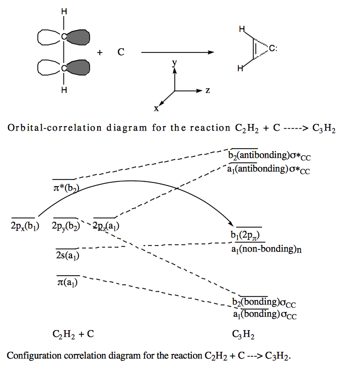
b. Forming SALC-AOs from the C and H atomic orbitals would generate the following:

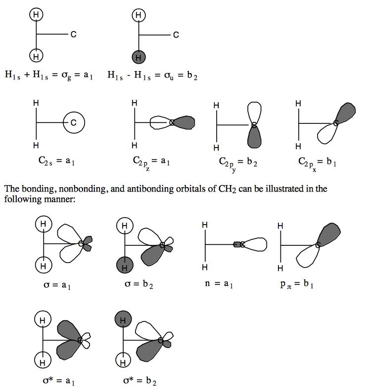
c.

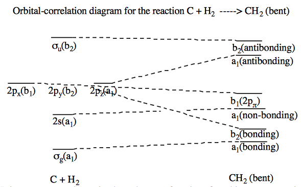
d. - e. It is necessary to determine how the wave functions found in part a. correlate with states of the \(CH_2\) molecule:
\begin{align} ^3P(xz,M_S=1); ^3B_1 &=& &\sigma_g^2s^2p_xp_z \longrightarrow sigma^2n^2p_\pi\sigma^{\text{*}} \\ ^3P(yx,M_S=1); ^3A_2 &=& &\sigma_g^2s^2p_xp_y \longrightarrow \sigma^2n^2p_\pi\sigma \\ ^3P(yz,M_S=1); ^3B_2 &=& &\sigma_g^2s^2p_yp_z \longrightarrow \sigma^2n^2\sigma\sigma^{\text{*}} \\ & & &^1D(xx-yy,M_S=0); ^1A_1 \longrightarrow \sigma^2n^2p_\pi^2 - \sigma^2n^2\sigma^2 \\ & & &^1D(yx,M_S=0); ^1A_2 \longrightarrow \sigma^2n^2\sigma p_\pi \\ & & &^1D(zx,M_S=0); ^1B_1 \longrightarrow \sigma^2n^2\sigma^{\text{*}}p_\pi \\ & & &^1D(zy,M_S=0); ^1B_2 \longrightarrow \sigma^2n^2\sigma^{\text{*}}\sigma \\ & & &^1D(2zz+xx+yy,M_S=0); ^1A_1 \longrightarrow 2\sigma^2n^2\sigma^{\text{*}2} + \sigma^2n^2p_{\pi}^2 + \sigma^2n^2\sigma^2 \end{align}
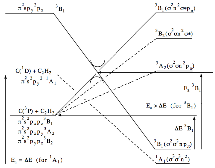
Note, the C + \(H_2\) state to which the lowest \(^1A_1 (\sigma^2n^2\sigma^2) CH_2\) state decomposes would be \( \sigma_g^2s^2p_y^2.\) This sate \((\sigma_g^2s^2p_y^2)\) cannon be obtained by a simple combination of the \(^1D\) states. In order to obtain pure \(\sigma_g^2s^2p_y^2)\) cannon be obtained by a simple combination of the \(^1D\) states. In order to obtain pure \(\sigma_g^2s^2p_y^2\) it is necessary to combine \( ^1S \text{ with } ^1D.\) For example,
\[ \sigma_g^2s^2p_y^2 = \dfrac{1}{6} \left( \sqrt{6} ^1D(0,0) - 2\sqrt{3} ^1S(0,0)\right) - \dfrac{1}{2} \left( ^1D(2,0) + ^1D(-2,0) \right). \nonumber \]
This indicates that a CCD must be drawn with a barrier near the \(^1D\) asymptote to represent the fact that \(^1A_1 \text{ CH}_2\) correlates with a mixture of \(^1D \text{ and } ^1S\) carbon plus hydrogen. The C + \(H_2\) state to which the lowest \(^3B_1 (\sigma^2n\sigma^2p_\pi )CH_2\) state decomposes would be \( \sigma_g^2sp_y^2p_x.\)

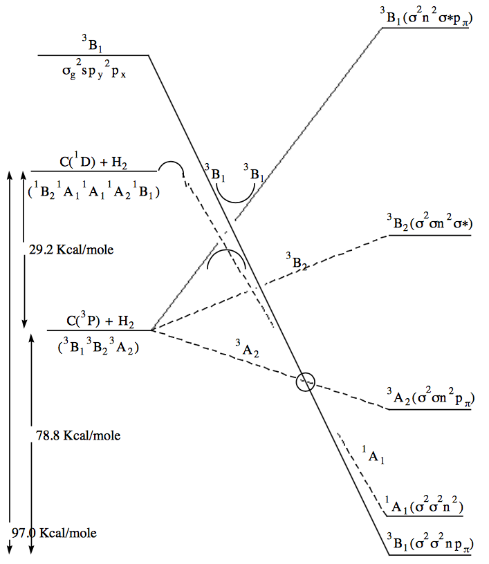
f. If you follow the \(^3B_1\) component of the \(C(^3P) + H_2\) (since it leads to the ground state products) to \(^3B_1 CH_2\) you must go over an approximately 20 Kcal/mole barrier. Of course this path produces \(^3B_1 CH_2\) product. Distortions away from \(C_{2v}\) symmetry, for example to \(C-s\) symmetry, would make the \(a_1 \text{ and } b_2\) orbitals identical in symmetry (a'). The \(b_1\) orbitals would maintain their identity group going to a" symmetry. Thus \(^3B_1 \text{ and } ^3A_2\) (both \(^3A" \text{ in } C_s\) symmetry and odd under reflection through the molecular plane) can mix. The system could thus follow the \(^3A_2\) component of the \(C(^3P) + H_2\) surface to the place (marked with a circle on the CCD) where it crosses the \(^3B_1\) surface upon which it then moves and continues to products. As a result, the barrier would be lowered.
You can estimate when the barrier occurs (late or early) using thermodynamic information for the reaction (i.e. slopes and asymptotic energies). For example, an early barrier would be obtained for a reaction with the characteristics:

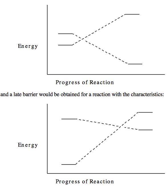
This relation between reaction endothermicity or exothermicity is known as the Hammond postulate. Note that the \( C(^3P_1) + H_2 \rightarrow CH_2\) reaction of interest here (see the CCD) has an early barrier.
g. The reaction \( C(^1D) + H_2 \rightarrow CH_2 (^1A_1)\) should have no symmetry barrier )this can be recognized by the following the \(^1A_1 (C(^1D) + H_2)\) reactants down to the \(^1A_1 (CH_2) \) products on the CCD).

Q2

This problem in many respects is analogous to problem 1.
The \(^3B_1\) surface certainly requires a two configuration CI wavefunction; the \(\sigma^2\sigma^2np_x (\pi^2p_y^2sp_x) \) and the \(\sigma^2n^2p_x\sigma^{\text{*}} (\pi^2s^2p_xp_z).\) The \( ^1A_1\) surface could use the \(sigma^2\sigma^2n^2 (\pi^2s^2p_y^2)\) only but once again there is n combination of \(^1D\) determinants which gives purely this configuration \((\pi^2s^2p_y^2)\). Thus mixing of both \(^1D \text{ and } ^1S\) determinants are necessary to yield the required \(pi^2s^2p_y^2\) configuration. Hence even the \(^1A_1\) surface would require a multiconfigurational wavefunction for adequate description.

Q3

a.
\begin{align} \langle \sigma_g | \sigma_g \rangle &=& & \langle \dfrac{1s_A + 1s_B}{\sqrt{2+2S}} \bigg| \dfrac{1s_A + 1s_B}{\sqrt{2+2S}} \rangle \\ &=& & \dfrac{1}{2+2S} \left( \langle 1s_A|1s_A\rangle + \langle 1s_A|1s_B \rangle + \langle 1s_B|1s_A \rangle + \langle 1s_B|1s_B \rangle \right) \\ &=& & (0.285)((1.000) + (0.753) + (0.753) + (1.000)) \\ &=& &0.999 \approx 1 \end{align}

\begin{align} \langle \sigma_g | \sigma_u \rangle &=& &\langle \dfrac{1s_A + 1s_B}{\sqrt{2+2S}} \bigg| \dfrac{1s_A - 1s_B}{\sqrt{2-2S}} \rangle \\ &=& &\dfrac{\langle 1s_A|1s_A \rangle + \langle 1s_A|1s_B \rangle + \langle 1s_B|1s_A \rangle + \langle 1s_B|1s_B \rangle}{\sqrt{2+2S}\sqrt{2-2S}} \\ &=& & (1.434)(0.534)((1.000) - (0.753) + (0.753) - (1.000)) \\ &=& &0 \\ \langle \sigma_u |\rangle &=& & \langle \dfrac{1s_A-1s_B}{\sqrt{2-2S}} \bigg| \dfrac{1s_A - 1s_B}{\sqrt{2-2S}}\rangle \\ &=& & \dfrac{\langle 1s_A|1s_A \rangle - \langle 1s_A|1s_B \rangle - \langle 1s_B|1s_A \rangle + \langle 1s_B|1s_B \rangle}{2-2S} \\ &=& &(2.024)((1.000) - (0.753) - (0.753) + (1.000)) \\ &=& & 1.000 \end{align}

b.
\begin{align} \langle \sigma_g|h|\sigma_g \rangle &=& &\langle \dfrac{1s_A + 1s_B}{\sqrt{2+2S}} \bigg| h \bigg| \dfrac{1s_A + 1s_B}{\sqrt{2+2S}} \rangle \\ &=& & \dfrac{\langle 1s_A |h|1s_A \rangle + \langle 1s_A|h|1s_B \rangle + \langle 1s_B|h|1s_A \rangle + \langle 1s_B|h|1s_B \rangle}{2+2S} \\ &=& & (0.285)((-1.110) + (-0.968) + (-0.968) + (-1.110)) \\ &=& & -1.184 \\ \langle \sigma_u |h| \sigma_u \rangle &=& & \langle \dfrac{1s_A - 1s_B}{\sqrt{2-2S}} \bigg| h \bigg| \dfrac{1s_A - 1s_B}{\sqrt{2-2S}} \rangle \\ &=& &\dfrac{\langle 1s_A |h|1s_A \rangle - \langle 1s_A|h|1s_B \rangle - \langle 1s_B|h|1s_A \rangle + \langle 1s_B|h|1s_B \rangle}{2-2S} \\ &=& &(2.024)((-1.110) + (0.968) + (0.968) + (-1.110)) \\ &=& &-0.575 \\ \langle \sigma_g\sigma_g |h|\sigma_g\sigma_g \rangle &\equiv & & \langle gg|gg\rangle = \dfrac{1}{2+2S}\dfrac{1}{2+2S} \\ & & & \langle (1s_A + 1s_B) (1s_A + 1s_B) (1s_A + 1s_B) (1s_A + 1s_B) \\ &=& & \dfrac{1}{(2+2S)^2} ( \langle AA|AA \rangle + \langle AA|AB \rangle + \langle AA|BA \rangle + \langle AA|BB \rangle + \langle AB|AA \rangle + \langle AB|AB \rangle + \langle AB|BA \rangle + \langle AB|BB \rangle + \\ & & & \langle BA|AA \rangle + \langle BA|AB \rangle + \langle BA|BA \rangle + \langle BA|BB \rangle + \langle BB|AA \rangle + \langle BB|BA \rangle + \langle BB|BA \rangle + \langle BB|BB \rangle ) \\ &=& & (0.081)((0.625) + (0.426) + (0.426) + (0.323) + (0.426) + (0.504) + (0.323) + (0.426) +\\ & & & (0.426) + (0.323) + (0.504) + (0.426) + (0.323) + (0.426) + (0.426) + (0.625)) \\ &=& &0.564 \\ \langle uu|uu \rangle &=& & \dfrac{1}{2-2S}\dfrac{1}{2-2S} \\ & & &\langle (1s_A - 1s_B) (1s_A - 1s_B)|(1s_A - 1s_B)(1s_A - 1s_B) \rangle \\ &=& &\dfrac{1}{(2-2S)^2} ( \langle AA|AA \rangle - \langle AA|AB \rangle - \langle AA|BA \rangle \langle AA|BB \rangle - \langle BA|AA \rangle + \langle BA|AB \rangle + \langle BA|BA \rangle - \langle BA|BB \rangle \\ & & & \langle BA|AA \rangle + \langle BA|AB \rangle + \langle BA|BA \rangle - \langle BA|BB \rangle + \langle BB|AA \rangle - \langle BB|AB \rangle - \langle BB|BA \rangle + \langle BB|BB \rangle ) \\ &=& &(4.100)((0.625) - (0.426) - (0.426) + (0.323) - (0.426) + (0.504) + (0.323) - (0.426) - \\ & & &(0.426) + (0.323) + (0.504) - (0.426) + (0.323) - (0.426) - (0.426) + (0.625)) \\ &=& & 0.582 \end{align}
\begin{align} \langle gg|uu \rangle &=& & \dfrac{1}{2+2S}\dfrac{1}{2-2S} \\ & & & \langle (1s_A + 1s_B)(1s_A + 1s_B)|(1s_A - 1s_B)(1s_A-1s_B) \rangle \\ &=& & \dfrac{1}{2+2S}\dfrac{1}{2-2S} \\ & & & ( \langle AA|AA \rangle - \langle AA|AB \rangle - \langle AA|BA \rangle + \langle AA|BB \rangle + \langle AB|AA \rangle - \langle AB|AB \rangle - \langle AB|BA \rangle + \langle AB|BB \rangle + \\ & & &+ \langle BA|AA \rangle - \langle BA|AB \rangle - \langle BA|BA \rangle + \langle BA|BB \rangle + \langle BB|AA \rangle - \langle BB|AB \rangle - \langle BB|BA \rangle + \langle BB|BB \rangle )\\ &=& & (0.285)(2.024)(( 0.625) - (0.426) - (0.426) + (0.323) + (0.426) - (0.504) - (0.323) + (0.426) + \\ & & &+ (0.426) - (0.323) - (0.504) - (0.426) + (0.323) - (0.426) - (0.426) + (0.625) \\ &=& &0.140 \\ \langle gu|gu \rangle &=& & \dfrac{1}{2+2S}\dfrac{1}{2-2S} \\ & & &\langle (1s_A + 1s_B)(1s_A - 1s_B)(1s_A + 1s_B)(1s_A - 1s_B) \rangle \\ &=& & \dfrac{1}{2+2S}\dfrac{1}{2-2S} \\ & & &( \langle AA|AA \rangle - \langle AA|AB \rangle + \langle AA|BA \rangle - \langle AA|BB \rangle - \langle AB|AA \rangle + \langle AB|AB \rangle - \langle AB|BA \rangle + \langle AB|BB \rangle \\ & & &+ \langle BA|AA \rangle - \langle BA|AB \rangle + \langle BA|BA \rangle - \langle BA|BB \rangle - \langle BB|AA \rangle + \langle BB|AB \rangle - \langle BB|BA \rangle + \langle BB|BB \rangle ) \\ &=& & (0.285)(2.024)((0.625) - (0.426) + (0.426) - (0.323) - (0.426) + (0.504) - (0.323) + (0.426) + ...\\ & & &...+ (0.426) - (0.323) + (0.504) - (0.426) - (0.323) + (0.426) - (0.426) + (0.625)) \\ &=& & 0.557 \end{align}

Note, that \( \langle gg|gu \rangle = \langle uu|ug \rangle = 0\) from symmetry considerations, but this can be easily verified. For example,
\begin{align} \langle gg|gu \rangle .&=& & \dfrac{1}{\sqrt{2+2S}}\dfrac{1}{\sqrt{(2-2S)^3}} \\ & & &\langle (1s_A + 1s_B)(1s_A + 1s_B) \bigg| (1s_A + 1s_B)(1s_A - 1s_B) \rangle \\ &=& & \dfrac{1}{\sqrt{2+2S}}\dfrac{1}{(2-2S)^3}. \\ & & & ( \langle AA | AA \rangle - \langle AA | AB \rangle + \langle AA | BA \rangle - \langle AA | BB \rangle \\ & & & \langle AB | AA \rangle - \langle AB | AB \rangle + \langle AB | BA \rangle - \langle AB | BB \rangle + \\ & & & \langle BA | AA \rangle - \langle BA | AB \rangle + \langle BA | BA \rangle - \langle BA | BB \rangle + \\ & & & \langle BB | AA \rangle - \langle BB | AB \rangle + \langle BB | BA \rangle - \langle BB | BB \rangle ) \\ & & & (0.534)(2.880)((0.625) - (0.426) + (0.426) - (0.323) + (0.426) - (0.504) + (0.323) - (0.426) +... \\ & & & ...+ (0.426) - (0.323) + (0.504) - (0.426) + (0.323) - (0.426) + (0.426) - (0.625)) \\ &=& & 0.000 \end{align}

c. We can now set up the configuration interaction Hamiltonian matrix. The elements are evaluated by using the Slater-Condon rules as shown in the text.
\begin{align} H_{11} &=& & \langle \sigma_g\alpha\sigma_g\beta |H| \sigma_g\alpha\sigma_g\beta \rangle \\ &=& &2f_{\sigma_g\sigma_g} + g_{\sigma_g\sigma_g\sigma_g\sigma_g} \\ &=& &2(-1.184) + 0.564 = -1.804 \\ H_{21} &=& &H_{12} = \langle \sigma_g\alpha\sigma_g\beta |H| \sigma_u\alpha\sigma_u\beta\rangle \\ &=& & g_{\sigma_g\sigma_g\sigma_u\sigma_u} \\ &=& & 0.140 \\ H_{22} &=& &\langle \sigma_u\alpha\sigma_u\beta |H| \sigma_u\alpha\sigma_u\beta\rangle \\ &=& & 2f_{\sigma_u\sigma_u} + g_{\sigma_u\sigma_u\sigma_u\sigma_u} \\ &=& & 2(-0.575) + 0.582 = -0.568 \end{align}

d. Solving this eigenvalue problem:
\begin{align} \begin{vmatrix} -1.804 - \varepsilon & 0.140 \\ 0.140 & -0.568 - \varepsilon \end{vmatrix} &=& & 0 \\ (-1.804 -\varepsilon)(-0.568 - \varepsilon) - (0.140)^2 &=& & 0 \\1.025 + 1.804\varepsilon + 0.568\varepsilon + \varepsilon^2 - 0.0196 &=& &0 \\ \varepsilon^2 + 2.372\varepsilon + 1.005 &=& &0 \\ \varepsilon &=& & \dfrac{-2.372 \pm \sqrt{(2.372)^2 - 4(1)(1.005)}}{(2)(1)}\\ &=& &-1.186 \pm 0.634 \\ &=& & -1.820, \text{ and } -0.552. \end{align}

Solving for the coefficients:
\begin{align}\begin{bmatrix} -1,804 - \varepsilon & 0.140 \\ 0.140 & -0.568 - \varepsilon \end{bmatrix}\begin{bmatrix} C_1 \\ C_2 \end{bmatrix} = \begin{bmatrix} 0 \\ 0 \end{bmatrix} \end{align}
For the first eigenvalue this becomes:
\begin{align} & & &\begin{bmatrix} -1.804 + 1.820 & 0.140 \\ 0.140 & -0.568 + 1.820 \end{bmatrix}\begin{bmatrix} C_1\\C_2 \end{bmatrix} = \begin{bmatrix}0\\0 \end{bmatrix} \\ & & & \begin{bmatrix} 0.016 & 0.140 \\ 0.140 & 1.252 \end{bmatrix}\begin{bmatrix} C_1 \\ C_2 \end{bmatrix} = \begin{bmatrix} 0 \\ 0 \end{bmatrix} \\& & & (0.140)(C_1) + (1.252)(C_2) = 0 \\ & & & C_1 = -8.943 C_2 \\ & & & C_1^2 + C_2^2 = 1 \text{(from normalization)} \\ & & & (-8.943 C_2)^2 + C_2^2 = 1 \\ & & & 80.975 C_2^2 = 1 \\ & & & C_2 = 0.111, C_1 = -0.994 \end{align}
For the second eigenvalue this becomes:
\begin{align} & & &\begin{bmatrix} -1.804 + 0.552 & 0.140 \\ 0.140 & -0.568 + 0.552 \end{bmatrix} \begin{bmatrix} C_1 \\ C_2 \end{bmatrix} = \begin{bmatrix} 0 \\ 0 \end{bmatrix} \\ & & & \begin{bmatrix} -1.252 & 0.140 \\ 0.140 & -0.016 \end{bmatrix}\begin{bmatrix} C_1 \\ C_2 \end{bmatrix} = \begin{bmatrix} 0 \\ 0 \end{bmatrix} \\ & & & (-1.252)(C_1) + (0.140)(C_2) \\ & & & C_1 = 0.112 C_2 \\ & & & C_1^2 + C_2^2 = 1\text{ (from normalization) } \\ & & & (0.112 C_2)^2 + C_2^2 = 1 \\ & & & 1.0125 C_2^2 = 1 \\ & & & C_2 = 0.994, C_1 = 0.111 \end{align}

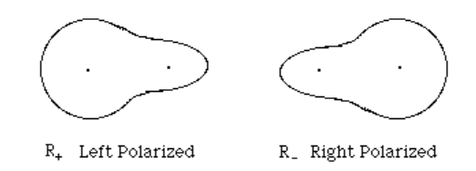
e. The polarized orbitals, \(R_{\pm}\), are given by:
\begin{align} R_{\pm} &=& & \sigma_g \pm \sqrt{\dfrac{C_2}{C_1}}\sigma_u \\ R_{\pm} &=& & \sigma_g \pm \sqrt{\dfrac{0.111}{0.994}}\sigma_u \\ R_{\pm} &=& & \sigma_g \pm 0.334 \sigma_u \\ R_{+} &=& & \sigma_g + 0.334 \sigma_u \text{ (left polarized) } \\ R_{-} &=& & \sigma_g - 0.334 \sigma_u \text{ (right polarized) }\end{align}