22.2.5: v. Exercise Solution

Last updated
Save as PDF

Page ID: 80355

\( \newcommand{\vecs}[1]{\overset { \scriptstyle \rightharpoonup} {\mathbf{#1}} } \) \( \newcommand{\vecd}[1]{\overset{-\!-\!\rightharpoonup}{\vphantom{a}\smash {#1}}} \)\(\newcommand{\id}{\mathrm{id}}\) \( \newcommand{\Span}{\mathrm{span}}\) \( \newcommand{\kernel}{\mathrm{null}\,}\) \( \newcommand{\range}{\mathrm{range}\,}\) \( \newcommand{\RealPart}{\mathrm{Re}}\) \( \newcommand{\ImaginaryPart}{\mathrm{Im}}\) \( \newcommand{\Argument}{\mathrm{Arg}}\) \( \newcommand{\norm}[1]{\| #1 \|}\) \( \newcommand{\inner}[2]{\langle #1, #2 \rangle}\) \( \newcommand{\Span}{\mathrm{span}}\) \(\newcommand{\id}{\mathrm{id}}\) \( \newcommand{\Span}{\mathrm{span}}\) \( \newcommand{\kernel}{\mathrm{null}\,}\) \( \newcommand{\range}{\mathrm{range}\,}\) \( \newcommand{\RealPart}{\mathrm{Re}}\) \( \newcommand{\ImaginaryPart}{\mathrm{Im}}\) \( \newcommand{\Argument}{\mathrm{Arg}}\) \( \newcommand{\norm}[1]{\| #1 \|}\) \( \newcommand{\inner}[2]{\langle #1, #2 \rangle}\) \( \newcommand{\Span}{\mathrm{span}}\)\(\newcommand{\AA}{\unicode[.8,0]{x212B}}\)

Two Slater type orbitals, i and j, centered on the same point results in the following overlap integrals:
\[ S_{ij} = \int\limits^{2\pi}_{0}\int\limits^{\pi}_0\int\limits^{\infty}_0 \left( \dfrac{2\xi_i}{a_0} \right)^{n_i+\dfrac{1}{2}}\sqrt{\dfrac{1}{(2n_i)!}} r^{(n_i-1)}e^{\left( \dfrac{-\xi_i r}{a_0} \right)} Y_{l_i,m_i}(\theta,\phi ) \left( \dfrac{2\xi_j}{a_0} \right)^{n_j+\dfrac{1}{2}} \sqrt{ \dfrac{1}{(2n_j)!}} r^{(n_j-1)}e^{\left( \dfrac{-\xi_j r}{a_0} \right)} Y_{l_j,m_j}(\theta,\phi ) r^2sin \theta drd\theta d\phi . \nonumber \]

For these s orbitals l = m = 0 and \( Y_{0,0}(\theta ,\phi ) = \dfrac{1}{\sqrt{4\pi}}. \) Performing the integrations over \(\theta\) and \(\phi\) yields \(4\pi\) which then cancels with these Y terms. The integral then recuces to:
\[ S_{ij} = \left( \dfrac{2\xi_i}{a_0} \right)^{n_i+\dfrac{1}{2}} \sqrt{\dfrac{1}{(2n_i)!}} \left( \dfrac{2\xi_j}{a_0} \right)^{n_j + \dfrac{1}{2}} \sqrt{\dfrac{1}{(2n_j)!}} \int\limits^{\infty}_{0} r^{(n_i-1+n_j-1)}e^{\left( \dfrac{-(\xi_i+\xi_j)r}{a_0} \right)}r^2dr \nonumber \]
\[ = \left( \dfrac{2\xi_i}{a_0} \right)^{n_i+\dfrac{1}{2}} \sqrt{\dfrac{1}{(2n_i)!}} \left( \dfrac{2\xi_j}{a_0} \right)^{n_j + \dfrac{1}{2}}\sqrt{\dfrac{1}{(2n_j)!}}\int\limits^{\infty}_{0} r^{(n_i-1+n_j-1)}e^{\left( \dfrac{-(\xi_i+\xi_j)r}{a_0} \right)}r^2dr \nonumber \]

Using integral equation (4) the integral then reduces to:

\[ S_{ij} = \left( \dfrac{2\xi_i}{a_0} \right)^{n_i + \dfrac{1}{2}} \sqrt{\dfrac{1}{(2n_i)!}} \left( \right)^{n_j+\dfrac{1}{2}} \sqrt{ \dfrac{1}{(2n_j)!}}(n_i+n_j)! \left( \dfrac{a_0}{\xi_i+\xi_j} \right)^{n_i+n_j+1}. \nonumber \]

We then substitute in the values for each of these constants:
\[ \text{for i=1; n=1, l=m=0, and } \xi = 2.6906 \nonumber \]
\[ \text{for i=2; n=2, l=m=0, and } \xi = 0.6396 \nonumber \]
\[ \text{for i=3; n=3, l=m=0, and } \xi = 0.1503. \nonumber \]

Evaluating each of these matrix elements we obtain:

\[ S_{11} = (12.482992)(0.707107)(12.482992)(0.707107)(2.00)(0.006417) = 1.000000 \nonumber \]
\[ S_{21}=S_{12} = (1.850743)(0.204124)(12.482992)(0.707107)(6.00)(0.008131) = 0.162673 \nonumber \]
\[ S_{22} = (1.850743)(0.204124)(1.850743)(0.204124)(24.00)(0.291950) = 1.00 \nonumber \]
\[ S_{31} = S_{13} = (0.0144892)(0.037268)(12.482992)(0.707107)(24.00)(0.005404) = 0.000635 \nonumber \]
\[ S_{32} = S_{23} = (0.014892)(0.037268)(1.850743)(0.204124)(120.00)(4.116872) = 0.103582 \nonumber \]
\[ S_{33} = (0.014892)(0.037268)(0.014892)(0.037268)(720.00)(4508.968136) = 1.00 \nonumber \]

\[ S = \begin{bmatrix} & 1.000000 & & & \\ & 0.162673 & 1.000000 & & \\ & 0.000635 & 0.103582 & 1.000000 & \end{bmatrix} \nonumber \]

We now solve the matrix eigenvalue problem S U = \(\lambda\) U.
The eigenvalues, \(\lambda\), of this overlap matrix are:
[ 0.807436 0.999424 1.193139 ],
and the corresponding eigenvectors, U, are:

\begin{bmatrix} & 0.596540 & -0.537104 & -0.596372 & \\ & -0.707634 & -0.001394 & 0.706578 & \\ & 0.378675 & 0.843515 & -0.380905 & \end{bmatrix}

The \(\lambda^{-\dfrac{1}{2}}\) matrix becomes:

\[ \lambda^{-\dfrac{1}{2}} = \begin{bmatrix} & 1.112874 & 0.000000 & 0.000000 & \\ & 0.000000 & 1.000288 & 0.000000 & \\ & 0.000000 & 0.000000 & 0.915492 & \end{bmatrix}. \nonumber \]

Back transforming into the original eigenbasis gives \( S^{-\dfrac{1}{2}}\), e.g.
\[ S^{-\dfrac{1}{2}} = U\lambda^{-\dfrac{1}{2}} U^T \nonumber \]
\[ S^{-\dfrac{1}{2}} = \begin{bmatrix} & 1.010194 & & & \\ & -0.083258 & 1.014330 & & \\ & 0.006170 & -0.052991 & 1.004129 & \end{bmatrix} \nonumber \]

The old ao matrix can be written as:

\[ C = \begin{bmatrix} & 1.000000 & 0.000000 & 0.000000 & \\ & 0.000000 & 1.000000 & 0.000000 & \\ & 0.000000 & 0.000000 & 1.000000 & \end{bmatrix} \nonumber \]

The new ao matrix (which now gives each ao as a linear combination of the original aos) then becomes:

\[ C^{\prime} = S^{-\dfrac{1}{2}}C = \begin{bmatrix} & 1.010194 & -0.083258 & 0.006170 & \\ & -0.083258 & 1.014330 & -0.052991 & \\ & 0.006170 & -0.052991 & 1.004129 & \end{bmatrix} \nonumber \]

These new aos have been constructed to meet the orthonormalization requirement \( C^{\prime T}SC^{\prime} = 1 \) since:

\[ \left( S^{-\dfrac{1}{2}}C \right)^T SS^{-\dfrac{1}{2}} C = C^TS^{-\dfrac{1}{2}} SS^{-\dfrac{1}{2}} C=C^TC = 1. \nonumber \]

But, it is always good to check our result and indeed:

\[ C^{\prime T}SC^{\prime} = \begin{bmatrix} & 1.000000 & 0.000000 & 0.000000 & \\ & 0.000000 & 1.000000 & 0.000000 & \\ & 0.000000 & 0.000000 & 1.000000 & \end{bmatrix} \nonumber \]
The least time consuming route here is to evaluate each of the needed integrals first. These are evaluated analogous to exercise 1, letting \(\chi_i\) denote each of the individual Slater Type Orbitals.

\[ \begin{align} \int\limits^{\infty}_{0} \chi_i r \chi_j r^2 dr & = & \langle r \rangle_{ij} \\ & = & \left( \dfrac{2\xi_i}{a_0} \right)^{n_i + \dfrac{1}{2}} \sqrt{\dfrac{1}{(2n_i)!}} \left( \dfrac{2\xi_j}{a_0} \right)^{n_j + \dfrac{1}{2}} \sqrt{\dfrac{1}{(2n_j)!}}\int\limits_{0}^{\infty}r^{(n_i+n_j+1)}e^{\left( -\dfrac{(\xi_i+\xi_j)r}{a_0} \right)}dr \end{align} \nonumber \]

Once again using integral equation (4) the integral recduces to:
\[ = \left( \dfrac{2\xi_i}{a_0} \right)^{n_i + \dfrac{1}{2}} \sqrt{\dfrac{1}{(2n_i)!}} \left( \dfrac{2\xi_j}{a_0} \right)^{n_j+\dfrac{1}{2}} \sqrt{\dfrac{1}{(2n_j)!}}\int\limits_0^{\infty}r^{(n_i+n_j+1)}e^{\left(-\dfrac{(\xi_i+\xi_j )r}{a_0}\right)}dr \nonumber \]

Again, upon substituting in the values for each of these constants, evaluation of these expectation values yields:

\[ \langle r \rangle_{11} = (12.482992)(0.707107)(12.482992)(0.707107)(6.00)(0.001193) = 0.557496 \nonumber \]
\[ \langle r \rangle_{21} = \langle r \rangle_{12} (1.850743)(0.204124)(12.482992)(0.707107)(24.00)(0.002441) = 0.195391 \nonumber \]
\[ \langle r \rangle_{22} = (1.850743)(0.204124)(1.850743)(0.204124)(120.00)(0.228228) = 3.908693 \nonumber \]
\[ \langle r \rangle_{31} = \langle r \rangle_{13} = (0.014892)(0.0337268)(12.482292)(0.707107)(120.00)(0.001902) = 0.001118 \nonumber \]
\[ \langle r \rangle_{32} = \langle r \rangle_{23} = (0.014892)(0.037268)(1.850743)(0.204124)(720.00)(5.211889) = 0.786798 \nonumber \]
\[ \langle r \rangle_{33} = (0.014892)(0.037268)(0.014892)(0.037268)(5040.00)(14999.893999) = 23.286760 \nonumber \]

\[ \int\limits_{0}^{\infty}\chi_i r\chi_j r^2 dr = \langle r \rangle_{ij} \begin{bmatrix} & 0.557496 & & & \\ & 0.195391 & 3.908693 & & \\ & 0.001118 & 0.786798 & 23.286760 & \end{bmatrix} \nonumber \]

Using these integrals one then proceeds to evaluate the expectation values of each of the orthogonalized aos, \( \chi^{\prime}_n\), as:
\[ \int\limits^{\infty}_{0} \chi^{\prime}_n r \chi^{\prime}_n r^2 dr = \sum\limits_{i=1}^3 \sum\limits_{j=1}^3 C^{\prime}_{ni}C_{nj}^{\prime} \langle r \rangle_{ij}. \nonumber \]
This results in the following expectation values (in atomic units):

\[ \begin{align} \int\limits_{0}^{\infty} \chi^{\prime}_{1s} r \chi^{\prime}_{1s} r^2 dr & = & 0.563240 \text{ bohr} \\ \int\limits_{0}^{\infty} \chi^{\prime}_{2s} r \chi^{\prime}_{2s} r^2 dr & = & 3.973199 \text{ bohr} \\ \int\limits_{0}^{\infty} \chi^{\prime}_{3s} r \chi^{\prime}_{3s} r^2 dr & = & 23.406622 \text{ bohr} \end{align} \nonumber \]
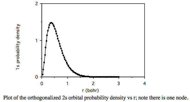
The radial density for each orthogonalized orbital, \( \chi^{\prime}_n\), assuming integrations over θ and \(\phi\) have already been performed can be written as:

\[ \int\limits_{0}^{\infty} \chi^{\prime}_n\chi^{\prime}_n r^2 dr = \sum\limits_{i=1}^3\sum\limits_{j=1}^3 C^{\prime}_{ni}C^{\prime}_{nj} \int\limits_{0}^{\infty} R_iR_j r^2 dr \text{ , where } R_i \text{ and } R_j \text{ are the radial portions of the individual Slater Type Orbitals, e.g.,} \nonumber \]

\[ R_iR_jr^2 = \left( \dfrac{2\xi_i}{a_0} \right)^{n_i + \dfrac{1}{2}}\sqrt{\dfrac{1}{(2n_i)!}}\left( \dfrac{2\xi_j}{a_0} \right)^{n_j+\dfrac{1}{2}}\sqrt{\dfrac{1}{(2n_j)!}}r^{(n_i+n_j)}e^{\left(-\dfrac{(\xi_i+\xi_j)r}{a_0} \right)} \nonumber \]

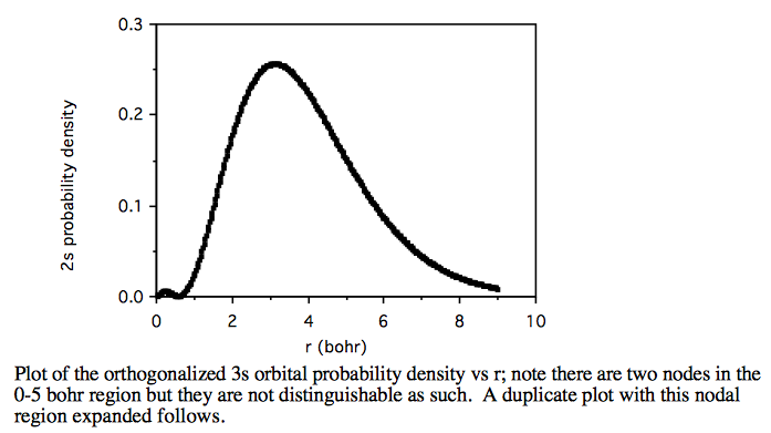
Therefore a plot of the radial probability for a given orthogonalized atomic orbital, n, will be: \( \sum\limits_{i=1}^3\sum\limits_{j=1}^3 C^{\prime}_{ni}C^{\prime}_{nj}R_iR_jr^2 \text{ vs. r.} \)

Plot the orthogonalized 1s orbital probability density vs r; note there are no nodes.