
12.3: Various Types of Configuration Mixing
- Page ID
- 63350

Essential CI
The above examples of the use of CCD's show that, as motion takes place along the proposed reaction path, geometries may be encountered at which it is essential to describe the electronic wavefunction in terms of a linear combination of more than one CSF:
\[ \Psi = \sum\limits_I C_I \Phi_I \nonumber \]
where the \(\Phi_I\)I are the CSFs which are undergoing the avoided crossing. Such essential configuration mixing is often referred to as treating "essential CI".
Dynamical CI
To achieve reasonable chemical accuracy (e.g., ± 5 kcal/mole) in electronic structure calculations it is necessary to use a multiconfigurational \(\Psi\) even in situations where no obvious strong configuration mixing (e.g., crossings of CSF energies) is present. For example, in describing the \(\pi^2\) bonding electron pair of an olefin or the \(ns^2\) electron pair in alkaline earth atoms, it is important to mix in doubly excited CSFs of the form \((\pi^{\text{*}})^2\) and \(np^2\), respectively. The reasons for introducing such a CI-level treatment were treated for an alkaline earth atom earlier in this chapter.
Briefly, the physical importance of such doubly-excited CSFs can be made clear by using the identity:
\[ C_I |..\phi\alpha \phi \beta ..| - C_2 |..\phi ' \alpha \phi ' \beta ..| \nonumber \]
\[ = \frac{C_I}{2}\left[ | ..(\phi - x\phi ')\alpha(\phi + x\phi ')\beta ..| - | ..(\phi - x\phi ')\beta (\phi + x\phi ')\alpha ..| \right], \nonumber \]
where
\[ x = \sqrt{\frac{C_2}{C_1}} \nonumber \]
This allows one to interpret the combination of two CSFs which differ from one another by a double excitation from one orbital \((\phi)\) to another \((\phi ')\) as equivalent to a singlet coupling of two different (non-orthogonal) orbitals \((\phi - x\phi ') \text{ and } (\phi + x\phi ')\). This picture is closely related to the so-called generalized valence bond (GVB) model that W. A. Goddard and his co-workers have developed (see W. A. Goddard and L. B. Harding, Annu. Rev. Phys. Chem. 29 , 363 (1978)). In the simplest embodiment of the GVB model, each electron pair in the atom or molecule is correlated by mixing in a CSF in which that electron pair is "doubly excited" to a correlating orbital. The direct product of all such pair correlations generates the GVB-type wavefunction. In the GVB approach, these electron correlations are not specified in terms of double excitations involving CSFs formed from orthonormal spin orbitals; instead, explicitly non-orthogonal GVB orbitals are used as described above, but the result is the same as one would obtain using the direct product of doubly excited CSFs.
In the olefin example mentioned above, the two non-orthogonal "polarized orbital pairs" involve mixing the \(\pi\) and \(\pi^{\text{*}}\) orbitals to produce two left-right polarized orbitals as depicted below:
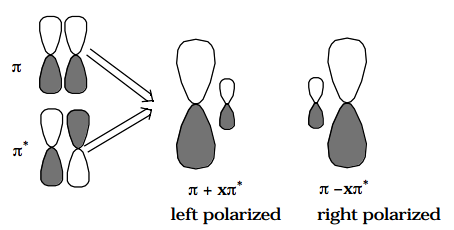
In this case, one says that the \(\pi^2\) electron pair undergoes left-right correlation when the \((\pi^{\text{*}})^2\) CSF is mixed into the CI wavefunction.
In the alkaline earth atom case, the polarized orbital pairs are formed by mixing the ns and np orbitals (actually, one must mix in equal amounts of \(p_1, p_{-1} , \text{ and }p_0 \text{ orbitals to preserve overall } ^1S\) symmetry in this case), and give rise to angular correlation of the electron pair. Use of an \((n+1)s^2\) CSF for the alkaline earth calculation would contribute in-out or radial correlation because, in this case, the polarized orbital pair formed from the ns and (n+1)s orbitals would be radially polarized.
The use of doubly excited CSFs is thus seen as a mechanism by which \(\Psi\) can place electron pairs , which in the single-configuration picture occupy the same orbital, into different regions of space (i.e., one into a member of the polarized orbital pair) thereby lowering their mutual coulombic repulsions. Such electron correlation effects are referred to as "dynamical electron correlation"; they are extremely important to include if one expects to achieve chemically meaningful accuracy (i.e., ± 5 kcal/mole).