2.5: Third-Order Nonlinear Spectroscopy

Now let’s look at examples of diagrammatic perturbation theory applied to third-order nonlinear spectroscopy. Third-order nonlinearities describe the majority of coherent nonlinear experiments that are used including pump-probe experiments, transient gratings, photon echoes, coherent anti-Stokes Raman spectroscopy (CARS), and degenerate four wave mixing (4WM). These experiments are described by some or all of the eight correlation functions contributing to \(R^{(3)}\):

\[R^{(3)}=\left(\frac{i}{\hbar}\right)^3\sum_{\alpha=1}^4\left[R_\alpha - R^*_\alpha\right] \label{3.5.1}\]

The diagrams and corresponding response first requires that we specify the system eigenstates. The simplest case, which allows us discuss a number of examples of third-order spectroscopy is a two-level system. Let’s write out the diagrams and correlation functions for a two-level system starting in \(\rho_{aa}\), where the dipole operator couples \(|b\rangle\) and \(|a\rangle\).

As an example, let’s write out the correlation function for R₂ obtained from the diagram above. This term is important for understanding photon echo experiments and contributes to pump-probe and degenerate four-wave mixing experiments.

\[\begin{aligned} R_{2} &=(-1)^{2} p_{a}\left(\mu_{b a}^{*}\right)\left[e^{-i \omega_{a b} \tau_{1}-\Gamma_{a b} \tau_{1}}\right]\left(\mu_{b a}\right)\left(e^{\cancel{-i \omega_{b b} \tau_{2}}-\Gamma_{b b} \tau_{2}}\right)\left(\mu_{a b}^{*}\right)\left[e^{-i \omega_{b a} \tau_{3}-\Gamma_{b a} \tau_{3}}\right]\left(\mu_{a b}\right) \\ &=p_{a}\left|\mu_{a b}\right|^{4} \exp \left[-i \omega_{b a}\left(\tau_{3}-\tau_{1}\right)-\Gamma_{b a}\left(\tau_{1}+\tau_{3}\right)-\Gamma_{b b}\left(\tau_{2}\right)\right] \end{aligned} \label{3.5.2}\]

The diagrams show how the input field contributions dictate the signal field frequency and wavevector. Recognizing the dependence of \(E_{sig}^{(3)} \sim P^{(3)} \sim R_2(E_1E_2E_3) \), these are obtained from the product of the incident field contributions

\[\begin{aligned} \bar E_1 \bar E_2 \bar E_3 &= \left(E_1^*e^{+i\omega_1t-i\bar k_1\cdot\bar r}\right)\left(E_2e^{-i\omega_2t+i\bar k_2\cdot r}\right)\left(E_3e^{+i\omega_3t-i\bar k_3\cdot\bar r_3}\right) \\ &\implies E_1^*E_2E_3e^{-\omega_{sig}t+i\bar k_{sig}\cdot\bar r} \end{aligned} \label{3.5.3}\]

\[\begin{aligned} \therefore \omega_{sig2} &= -\omega_1 + \omega_2 + \omega_3 \\ k_{sig2} &= -\bar k_1 +\bar k_2 +\bar k_3 \end{aligned} \label{3.5.4}\]

Now, let’s compare this to the response obtained from R₄. These we obtain

\[R_4=p_a|\mu_{ab}|^4exp\left[-i\omega_{ba}(\tau_3+\tau_1)-\Gamma_{ba}(\tau_1+\tau_3)-\Gamma_{bb}(\tau_2)\right] \label{3.5.5}\]

\[\begin{aligned} \omega_{sig4} &= +\omega_1 - \omega_2 + \omega_3 \\ k_{sig4} &= +\bar k_1 -\bar k_2 +\bar k_3 \end{aligned} \label{3.5.6}\]

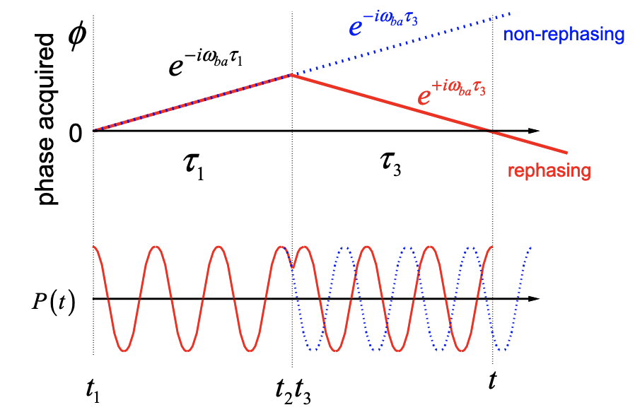
Note that R₂ and R₄ terms are identical, except for the phase acquired during the initial period: \(exp[i\phi]=exp[\pm i\omega_{ba}\tau_1]\). The R₂ term evolves in conjugate coherences during the \(\tau_1\) and \(\tau_3\) periods, whereas the R₄ term evolves in the same coherence state during both periods:

	Coherences in \(\tau_1\) and \(\tau_3\)	Phase acquired in \(\tau_1\) and \(\tau_3\)
R4	\(|b\rangle\langle a| \rightarrow |b\rangle\langle a| \)	\( e^{-i\omega_{ba}(\tau_1+\tau_3)} \)
R2	\(|a\rangle\langle b| \rightarrow |b\rangle\langle a|\)	\( e^{-i\omega_{ba}(\tau_1-\tau_3)} \)

The R₂ term has the property of time-reversal: the phase acquired during \(\tau_1\) is reversed in \(\tau_3\). For that reason the term is called “rephasing.” Rephasing signals are selected in photon echo experiments and are used to distinguish line broadening mechanisms and study spectral diffusion. For R₄, the phase acquired continuously in \(\tau_1\) and \(\tau_3\), and this term is called “nonrephasing.” Analysis of R₁ and R₃ reveals that these terms are non-rephasing and rephasing, respectively.

For the present case of a third-order spectroscopy applied to a two-level system, we observe that the two rephasing functions R₂ and R₃ have the same emission frequency and wavevector, and would therefore both contribute equally to a given detection geometry. The two terms differ in which population state they propagate during the \(\tau_2\) variable. Similarly, the non-rephasing functions R₁ and R₄ each have the same emission frequency and wavevector, but differ by the \(\tau_2\) population. For transitions between more than two system states, these terms could be separated by frequency or wavevector (see appendix). Since the rephasing pair R₂ and R₃ both contribute equally to a signal scattered in the −k₁ + k₂ + k₃ direction, they are also referred to as \(S_I\). The nonrephasing pair R1 and R4 both scatter in the + k₁ − k₂ + k₃ direction and are labeled as \(S_{II}\).

Our findings for the four independent correlation functions are summarized below.

			\(\omega_{sig}\)	\(k_{sig}\)	\(\tau_2\) population
\(S_I\)	rephasing	R2	\(-\omega_1 +\omega_2 +\omega_3\)	\(-k_1 +k_2 +k_3\)	excited state
		R3	\(-\omega_1 +\omega_2 +\omega_3\)	\(-k_1 +k_2 +k_3\)	ground state
\(S_{II}\)	non-rephasing	R1	\(+\omega_1 -\omega_2 +\omega_3\)	\(+k_1 -k_2 +k_3\)	ground state
		R4	\(+\omega_1 -\omega_2 +\omega_3\)	\(+k_1 -k_2 +k_3\)	excited state