1.2: Nonlinear Polarization

For nonlinear spectroscopy, we will calculate the polarization arising from interactions with multiple fields. We will use a perturbative expansion of \(P\) in powers of the incoming fields

\[\bar P(t)=P^{(0)}+P^{(1)}+P^{(2)}+\cdots\]

where \(P^{(n)}\) refers to the polarization arising from \(n\) incident light fields. So, \(P^{(2)}\) and higher are the nonlinear terms. We calculate P from the density matrix

\[\begin{align*} \bar P(t) &=Tr\left(\bar\mu_I(t)\rho_I(t)\right) \\[4pt] &=Tr\left(\bar\mu_I\rho_I^{(0)}\right)+Tr\left(\bar\mu_I\rho_I^{(1)}(t)\right)+Tr\left(\bar\mu_I\rho_I^{(2)}(t)\right)+\cdots \end{align*}\]

As we wrote earlier, \(P_I^{(n)}\) is the n^th order expansion of the density matrix

\[\rho^{(0)}=\rho_{eq}\nonumber\]

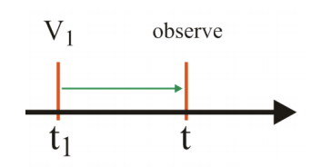
\[\rho^{(1)}=-\frac{i}{\hbar}\int\limits_{-\infty}^tdt_1\left[V_I(t_I),\rho_{eq}\right]\]

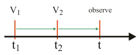
\[\rho^{(2)}=\left(-\frac{i}{\hbar}\right)^2\int\limits_{-\infty}^tdt_2\int\limits_{-\infty}^{t_2}dt_1\left[V_I(t_2)\left[V_I(t_I),\rho_{eq}\right]\right]\nonumber\]

\[\rho_I^{(n)}=\left(-\frac{i}{\hbar}\right)^n\int\limits_{-\infty}^{t}dt_n\int\limits_{-\infty}^{t_n}dt_{n-1}\cdots\int\limits_{-\infty}^{t_2}dt_1\left[V_I(t_n),\left[V_I(t_{n-1}),\left[\cdots\left[V_I(t_1),\rho_{eq}\right]\cdots\right]\right]\right]\]

Let’s examine the second-order polarization in order to describe the nonlinear response function. Earlier we stated that we could write the second-order nonlinear response arise from two time-ordered interactions with external potentials in the form

\[\bar P^{(2)}(t)=\int\limits_0^{\infty}d\tau_2\int\limits_0^{\infty}d\tau_1R^{(2)}\left(\tau_2,\tau_1\right)\bar E_1\left(t-\tau_2-\tau_1\right)\bar E_2\left(t-\tau_2\right)\]

We can compare this result to what we obtain from \(P^{(2)}(t)=Tr\left(\mu_I(t)\rho_I^{(2)}(t)\right)\). Substituting as we did in the linear case,

\[ \begin{aligned}
P^{(2)}(t) &=\operatorname{Tr}\left\{\mu_{I}(t)\left(-\frac{i}{\hbar}\right)^{2} \int_{-\infty}^{t} d t_{2} \int_{-\infty}^{t_{2}} d t_{1}\left[V_{I}\left(t_{2}\right),\left[V_{I}\left(t_{1}\right), \rho_{e q}\right]\right]\right\} \\
&=\left(\frac{i}{\hbar}\right)^{2} \int_{-\infty}^{t} d t_{2} \int_{-\infty}^{t_{2}} d t_{1} E_{2}\left(t_{2}\right) E_{1}\left(t_{1}\right) \operatorname{Tr}\left\{\left[\left[\mu_{I}(t), \mu_{I}\left(t_{2}\right)\right], \mu_{I}\left(t_{1}\right)\right] \rho_{e q}\right\} \\
&=\left(\frac{i}{\hbar}\right)^{2} \int_{0}^{\infty} d \tau_{2} \int_{0}^{\infty} d \tau_{1} E_{2}\left(t-\tau_{2}\right) E_{1}\left(t-\tau_{2}-\tau_{1}\right) \operatorname{Tr}\left\{\left[\left[\mu_{I}\left(\tau_{1}+\tau_{2}\right), \mu_{I}\left(\tau_{1}\right)\right], \mu_{I}(0)\right] \rho_{e q}\right\}
\end{aligned} \label{2.2.5} \]

In the last line we switched variables to the time-intervals \(t_1=t-\tau_1-\tau_2\) and \(t_2=t-\tau_2\), and enforced the time-ordering \(t_1 \le t_2\). Comparison of eqs. (2.2.4) and (2.2.5) allows us to state that the second order nonlinear response function is

\[ R^{(2)}\left(\tau_{1}, \tau_{2}\right)=\left(\frac{i}{\hbar}\right)^{2} \theta\left(\tau_{1}\right) \theta\left(\tau_{2}\right) \operatorname{Tr}\left\{\left[\left[\mu_{I}\left(\tau_{1}+\tau_{2}\right), \mu_{I}\left(\tau_{1}\right)\right], \mu_{I}(0)\right] \rho_{e q}\right\} \label{2.2.6} \]

Again, for impulsive interactions (i.e., delta function light pulses), the nonlinear polarization is directly proportional to the response function. Similar exercises to the linear and second order response can be used to show that the nonlinear response function to arbitrary order \(R^{(n)}\) is

\[\begin{aligned}
R^{(n)}\left(\tau_{1}, \tau_{2}, \ldots \tau_{n}\right) &=\left(\frac{i}{\hbar}\right)^{n} \theta\left(\tau_{1}\right) \theta\left(\tau_{2}\right) \ldots \theta\left(\tau_{n}\right) \\
& \times \operatorname{Tr}\left\{\left[\left[\ldots\left[\mu_{I}\left(\tau_{n}+\tau_{n-1}+\ldots+\tau_{1}\right), \mu_{I}\left(\tau_{n-1}+\tau_{n}+\cdots \tau_{1}\right)\right], \ldots\right] \mu_{I}(0)\right] \rho_{e q}\right\}
\end{aligned} \label{2.2.7} \]

We see that in general the nonlinear response functions are sums of correlation functions, and the n^th order response has 2n correlation functions contributing. These correlation functions differ by whether sequential operators act on the bra or ket side of ρ when enforcing the time-ordering. Since the bra and ket sides represent conjugate wavefunctions, these correlation functions will contain coherences with differing phase relationships during subsequent time-intervals.

To see more specifically what a specific term in these nested commutators refers to, let’s look at \(R^{(2)}\) and enforce the time-ordering:

Term 1 in eq. (2.2.7)

\[\begin{aligned} Q_1 &= Tr\left(\mu_1(\tau_1+\tau_2)\mu_I(\tau_1)\mu_I(0)\rho_{eq}\right) \\ &= Tr\left(\frac{U_0^{\dagger}(\tau_1+\tau_2)}{U_0^{\dagger}(\tau_1)U_0^{\dagger}(\tau_2)}\mu\frac{U_0(\tau_1+\tau_2)U_0^{\dagger}(\tau)}{U_0(\tau_2)}\mu U_0(\tau_1)\mu\rho_{eq}\right) \\ &=Tr\left(\mu U_0(\tau_2)\mu U_0(\tau_1)\mu\rho_{eq}U_0^{\dagger}(\tau_1)U_0^{\dagger}(\tau_2)\right) \end{aligned} \]

(1) dipole acts on ket of \(\rho_{eq}\)

(2) evolve under \(H_0\) during \(\tau_1\).

(3) dipole acts on ket.

(4) Evolve during \(\tau_2\).

(5) Multiply by \(\mu\) and take trace.

KET/KET interaction

At each point of interaction with the external potential, the dipole operator acted on ket side of ρ . Different correlation functions are distinguished by the order that they act on bra or ket. We only count the interactions with the incident fields, and the convention is that the final operator that we use prior to the trace acts on the ket side. So the term Q₁ is a ket/ket interaction. An alternate way of expressing this correlation function is in terms of the time-propagator for the density matrix, a superoperator defined through: \(\hat G(t)\rho_{ab}=U_0|a\rangle\langle b|U_0^{\dagger}\). Remembering the time-ordering, this allows Q₁ to be written as

\[Q_1 = Tr\left(\mu\hat G(\tau_2)\mu\hat G(\tau_1)\mu\rho_{eq}\right) \label{2.2.8}\]

Term 2

\[\begin{aligned} Q_2 &=Tr\left(\mu_I(0)\mu_I(\tau_1+\tau_2)\mu_I(\tau_1)\rho_{eq}\right) \\ &=Tr\left(\mu_I(\tau_1+\tau_2)\mu_I(\tau_1)\rho_{eq}\mu_I(0)\right) \end{aligned}\nonumber\]

BRA/KET interaction

For the remaining terms we note that the bra side interaction is the complex conjugate of ket side, so of the four terms in eq. (2.2.7), we can identify only two independent terms:

\[Q_1 \Rightarrow ket/ket ~~~~~ Q_1^* \Rightarrow bra/bra ~~~~~ Q_2 \Rightarrow ket/bra ~~~~~ Q_2^* \Rightarrow bra/ket \nonumber\]

This is a general observation. For \(R^{(n)}\), you really only need to calculate 2^n-1 correlation functions. So for \(R^{(2)}\) we write

\[R^{(2)}=\left(\frac{i}{\hbar}\right)^{2} \theta\left(\tau_{1}\right) \theta\left(\tau_{2}\right) \sum_{\alpha=1}^{2}\left[Q_{\alpha}\left(\tau_{1}, \tau_{2}\right)-Q_{\alpha}^{*}\left(\tau_{1}, \tau_{2}\right)\right] \label{2.2.9}\]

where

\[Q_1=Tr\left[\mu_I(\tau_1+\tau_2)\mu_I(\tau_1)\mu_I(0)\rho_{eq}\right] \label{2.2.10}\]

\[Q_1=Tr\left[\mu_I(\tau_1)\mu_I(\tau_1+\tau_2)\mu_I(0)\rho_{eq}\right] \label{2.2.11}\]

So what is the difference in these correlation functions? Once there is more than one excitation field, and more than one time period during which coherences can evolve, then one must start to carefully watch the relative phase that coherences acquire during different consecutive time-periods, \(\phi(\tau)=\omega_{ab}\tau\). To illustrate, consider wavepacket evolution: light interaction can impart positive or negative momentum (\(\pm\bar k_{in}\)) to the evolution of the wavepacket, which influences the direction of propagation and the phase of motion relative to other states. Any subsequent field that acts on this state must account for time-dependent overlap of these wavepackets with other target states. The different terms in the nonlinear response function account for all of the permutations of interactions and the phase acquired by these coherences involved. The sum describes the evolution including possible interference effects between different interaction pathways.