1.6: Phase space distribution functions and Liouville's theorem

Given an ensemble with many members, each member having a different phase space vector \(x\) corresponding to a different microstate, we need a way of describing how the phase space vectors of the members in the ensemble will be distributed in the phase space. That is, if we choose to observe one particular member in the ensemble, what is the probability that its phase space vector will be in a small volume \(dx\) around a point \(x\) in the phase space at time \(t\). This probability will be denoted

\[ f (x,t) dx \nonumber \]

where \(f (x, t)\) is known as the phase space probability density or phase space distribution function. It's properties are as follows:

\[f (x, t ) \ge (0 \nonumber \]

\(\int dx f (x, t)\) = Number of members in the ensemble

Liouville's Theorem

The total number of systems in the ensemble is a constant. What restrictions does this place on \(f (x, t ) \)? For a given volume \(\Omega \) in phase space, this condition requires that the rate of decrease of the number of systems from this region is equal to the flux of systems into the volume.

Let \(\hat {n} \) be the unit normal vector to the surface of this region.

Figure \(\PageIndex{1}\): Divergence through a surface

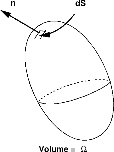
The flux through the small surface area element, \(dS\) is just \(\hat {n}\cdot \dot {x}f(x,t)dS \). Then the total flux out of volume is obtained by integrating this over the entire surface that encloses \(\Omega \):

\[\int dS \hat {n} \cdot (\dot {x} f(x,t)) = \int_{\Omega}\nabla _{x}\cdot(\dot{x} f(x,t)) \nonumber \]

which follows from the divergence theorem. \(\nabla _x\) is the \(6N\) dimensional gradient on the phase space

\[\nabla _x = \left(\frac {\partial}{\partial p_1},\cdots,\frac {\partial}{\partial p_N}, \frac {\partial}{\partial r_1},\cdots, \frac {\partial}{\partial r_N}\right) \nonumber \]

\[=\left(\nabla_{p_1},\cdots,\nabla_{p_N},\nabla_{r_1},\cdots,\nabla_{r_N}\right) \nonumber \]

On the other hand, the rate of decrease in the number of systems out of the volume is

\[-\frac {d}{dt}\int_{\Omega} d{x}f(x,t) = -\int_{\Omega}d{x} \frac {\partial}{\partial t} f(x,t) \nonumber \]

Equating these two quantities gives

\[ \int_{\Omega} dx \nabla_{x} \cdot (\dot{x}f( x,t)) = -\int_{\Omega} d{x} \frac {\partial}{\partial t}f(x,t) \nonumber \]

But this result must hold for any arbitrary choice of the volume \(\Omega \), which we may also allow to shrink to 0 so that the result holds locally, and we obtain the local result:

\[ \frac {\partial}{\partial t}f(x,t) + \nabla_{x} \cdot (\dot {x} f(x,t)) = 0 \nonumber \]

But

\[ \nabla _{x} \cdot (\dot {x} f (x,t)) = \dot {x} \cdot \nabla _x f(x,t) + f(x,t) \nabla _{x} \cdot \dot {x} \nonumber \]

This equation resembles an equation for a "hydrodynamic'' flow in the phase space, with \(f (x, t )\) playing the role of a density. The quantity \(\nabla _x \cdot \dot {x} \), being the divergence of a velocity field, is known as the phase space compressibility, and it does not, for a general dynamical system, vanish. Let us see what the phase space compressibility for a Hamiltonian system is:

\[\nabla_{x}\cdot\dot{x} = \sum_{i=1}^{N}\left[\nabla _{p_i} \cdot \dot {p} _i + \nabla_{r_i}\cdot \dot{r}_i \right] \nonumber \]

However, by Hamilton's equations:

\[ \dot {p}_i = -\nabla_{r_i}H\;\;\;\;\;\;\;\;\;\;\;\;\;\;\;\;\;\;\;\;\dot{r}_i = \nabla_{p_i}H \nonumber \]

Thus, the compressibility is given by

\[ \nabla_{x}\cdot\dot{x} =\sum_{i=1}^N \left[-\nabla _{p_i} \cdot \nabla _{r_i}H +\nabla_{r_i}\cdot\nabla_{p_i}H\right] = 0 \nonumber \]

Thus, Hamiltonian systems are incompressible in the phase space, and the equation for \(f (x, t )\) becomes

\[ \frac {\partial}{\partial t}f(x,t) + \dot{x}\cdot \nabla_{x}f(x,t) = \frac {df}{dt} = 0 \nonumber \]

which is Liouville's equation, and it implies that \(f (x, t )\) is a conserved quantity when \(x\) is identified as the phase space vector of a particular Hamiltonian system. That is, \(f (x_t, t)\) will be conserved along a particular trajectory of a Hamiltonian system. However, if we view \(x\) is a fixed spatial label in the phase space, then the Liouville equation specifies how a phase space distribution function \(f (x, t )\) evolves in time from an initial distribution \(f (x, 0 )\).