
2.5D: Quantitating with GC
- Page ID
- 95704

\( \newcommand{\vecs}[1]{\overset { \scriptstyle \rightharpoonup} {\mathbf{#1}} } \)
\( \newcommand{\vecd}[1]{\overset{-\!-\!\rightharpoonup}{\vphantom{a}\smash {#1}}} \)
\( \newcommand{\id}{\mathrm{id}}\) \( \newcommand{\Span}{\mathrm{span}}\)
( \newcommand{\kernel}{\mathrm{null}\,}\) \( \newcommand{\range}{\mathrm{range}\,}\)
\( \newcommand{\RealPart}{\mathrm{Re}}\) \( \newcommand{\ImaginaryPart}{\mathrm{Im}}\)
\( \newcommand{\Argument}{\mathrm{Arg}}\) \( \newcommand{\norm}[1]{\| #1 \|}\)
\( \newcommand{\inner}[2]{\langle #1, #2 \rangle}\)
\( \newcommand{\Span}{\mathrm{span}}\)
\( \newcommand{\id}{\mathrm{id}}\)
\( \newcommand{\Span}{\mathrm{span}}\)
\( \newcommand{\kernel}{\mathrm{null}\,}\)
\( \newcommand{\range}{\mathrm{range}\,}\)
\( \newcommand{\RealPart}{\mathrm{Re}}\)
\( \newcommand{\ImaginaryPart}{\mathrm{Im}}\)
\( \newcommand{\Argument}{\mathrm{Arg}}\)
\( \newcommand{\norm}[1]{\| #1 \|}\)
\( \newcommand{\inner}[2]{\langle #1, #2 \rangle}\)
\( \newcommand{\Span}{\mathrm{span}}\) \( \newcommand{\AA}{\unicode[.8,0]{x212B}}\)
\( \newcommand{\vectorA}[1]{\vec{#1}} % arrow\)
\( \newcommand{\vectorAt}[1]{\vec{\text{#1}}} % arrow\)
\( \newcommand{\vectorB}[1]{\overset { \scriptstyle \rightharpoonup} {\mathbf{#1}} } \)
\( \newcommand{\vectorC}[1]{\textbf{#1}} \)
\( \newcommand{\vectorD}[1]{\overrightarrow{#1}} \)
\( \newcommand{\vectorDt}[1]{\overrightarrow{\text{#1}}} \)
\( \newcommand{\vectE}[1]{\overset{-\!-\!\rightharpoonup}{\vphantom{a}\smash{\mathbf {#1}}}} \)
\( \newcommand{\vecs}[1]{\overset { \scriptstyle \rightharpoonup} {\mathbf{#1}} } \)
\( \newcommand{\vecd}[1]{\overset{-\!-\!\rightharpoonup}{\vphantom{a}\smash {#1}}} \)
\(\newcommand{\avec}{\mathbf a}\) \(\newcommand{\bvec}{\mathbf b}\) \(\newcommand{\cvec}{\mathbf c}\) \(\newcommand{\dvec}{\mathbf d}\) \(\newcommand{\dtil}{\widetilde{\mathbf d}}\) \(\newcommand{\evec}{\mathbf e}\) \(\newcommand{\fvec}{\mathbf f}\) \(\newcommand{\nvec}{\mathbf n}\) \(\newcommand{\pvec}{\mathbf p}\) \(\newcommand{\qvec}{\mathbf q}\) \(\newcommand{\svec}{\mathbf s}\) \(\newcommand{\tvec}{\mathbf t}\) \(\newcommand{\uvec}{\mathbf u}\) \(\newcommand{\vvec}{\mathbf v}\) \(\newcommand{\wvec}{\mathbf w}\) \(\newcommand{\xvec}{\mathbf x}\) \(\newcommand{\yvec}{\mathbf y}\) \(\newcommand{\zvec}{\mathbf z}\) \(\newcommand{\rvec}{\mathbf r}\) \(\newcommand{\mvec}{\mathbf m}\) \(\newcommand{\zerovec}{\mathbf 0}\) \(\newcommand{\onevec}{\mathbf 1}\) \(\newcommand{\real}{\mathbb R}\) \(\newcommand{\twovec}[2]{\left[\begin{array}{r}#1 \\ #2 \end{array}\right]}\) \(\newcommand{\ctwovec}[2]{\left[\begin{array}{c}#1 \\ #2 \end{array}\right]}\) \(\newcommand{\threevec}[3]{\left[\begin{array}{r}#1 \\ #2 \\ #3 \end{array}\right]}\) \(\newcommand{\cthreevec}[3]{\left[\begin{array}{c}#1 \\ #2 \\ #3 \end{array}\right]}\) \(\newcommand{\fourvec}[4]{\left[\begin{array}{r}#1 \\ #2 \\ #3 \\ #4 \end{array}\right]}\) \(\newcommand{\cfourvec}[4]{\left[\begin{array}{c}#1 \\ #2 \\ #3 \\ #4 \end{array}\right]}\) \(\newcommand{\fivevec}[5]{\left[\begin{array}{r}#1 \\ #2 \\ #3 \\ #4 \\ #5 \\ \end{array}\right]}\) \(\newcommand{\cfivevec}[5]{\left[\begin{array}{c}#1 \\ #2 \\ #3 \\ #4 \\ #5 \\ \end{array}\right]}\) \(\newcommand{\mattwo}[4]{\left[\begin{array}{rr}#1 \amp #2 \\ #3 \amp #4 \\ \end{array}\right]}\) \(\newcommand{\laspan}[1]{\text{Span}\{#1\}}\) \(\newcommand{\bcal}{\cal B}\) \(\newcommand{\ccal}{\cal C}\) \(\newcommand{\scal}{\cal S}\) \(\newcommand{\wcal}{\cal W}\) \(\newcommand{\ecal}{\cal E}\) \(\newcommand{\coords}[2]{\left\{#1\right\}_{#2}}\) \(\newcommand{\gray}[1]{\color{gray}{#1}}\) \(\newcommand{\lgray}[1]{\color{lightgray}{#1}}\) \(\newcommand{\rank}{\operatorname{rank}}\) \(\newcommand{\row}{\text{Row}}\) \(\newcommand{\col}{\text{Col}}\) \(\renewcommand{\row}{\text{Row}}\) \(\newcommand{\nul}{\text{Nul}}\) \(\newcommand{\var}{\text{Var}}\) \(\newcommand{\corr}{\text{corr}}\) \(\newcommand{\len}[1]{\left|#1\right|}\) \(\newcommand{\bbar}{\overline{\bvec}}\) \(\newcommand{\bhat}{\widehat{\bvec}}\) \(\newcommand{\bperp}{\bvec^\perp}\) \(\newcommand{\xhat}{\widehat{\xvec}}\) \(\newcommand{\vhat}{\widehat{\vvec}}\) \(\newcommand{\uhat}{\widehat{\uvec}}\) \(\newcommand{\what}{\widehat{\wvec}}\) \(\newcommand{\Sighat}{\widehat{\Sigma}}\) \(\newcommand{\lt}{<}\) \(\newcommand{\gt}{>}\) \(\newcommand{\amp}{&}\) \(\definecolor{fillinmathshade}{gray}{0.9}\)Quantitative Challenges
Most modern GC instruments allow for integration of the peaks in a GC spectrum with the click of a button. If an older instrument is used, triangulation may be used to calculate the area under a peak, or the peaks may be cut out from a paper spectrum and weighed on an analytical balance to integrate. Peak integrations are useful because it is possible to correlate the area under a peak to the quantity of material present in a sample. Note it is the area of a peak that is relevant, not the height. A tall, narrow peak may have a smaller area than a short, wide one. It would be very useful if peak areas would directly reflect mixture composition, but that is unfortunately not always the case. The reason for this has to do with how compounds are detected upon exit from a column.
Common detectors at undergraduate institutions are flame-ionization detectors (FID) and mass spectrometry detectors (MS). With an FID, a sample is ignited upon exit from the column, and the ions produced in the flame are "counted" by the amount of electric current. Unfortunately, different compounds produce different amounts of ions when burned, meaning the ion count will not be directly equivalent to the molar quantity. Similarly, a mass spectrometer counts the number of ions produced from all the fragments detected in the instrument (called the "Total Ion Count", TIC, the y-axis on Figure 2.84), which does not always directly represent the quantity of the original material. Some compounds fragment more than others in a mass spectrometer, causing them to be detected in a manner that does not represent their true abundance.
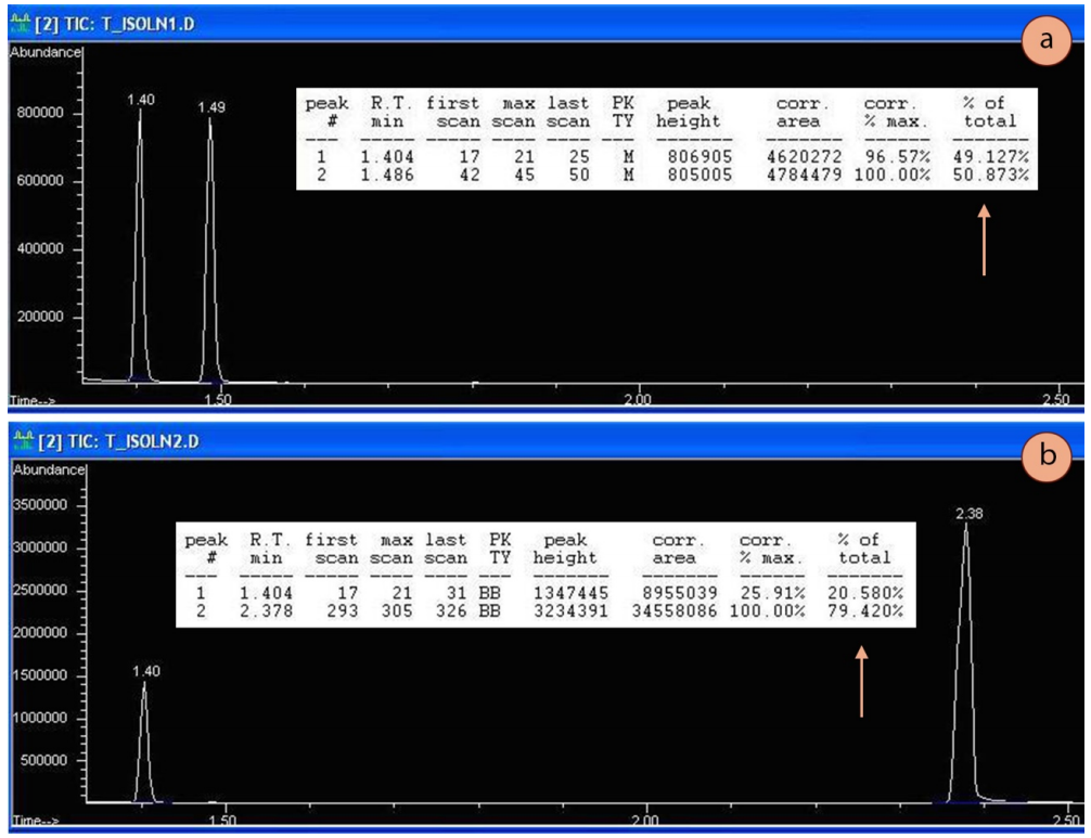
To demonstrate how peak integration does not always correlate with actual abundance, GC spectra of two samples containing equimolar quantities of two compounds is shown in Figure 2.84. Figure 2.84a contains equal molar amounts of 1-butanol and 2-butanol, while Figure 2.84b contains equal molar amounts of 2-butanol and 1-heptanol.
The area under the peaks was tabulated by the mass spectrometer (represented by the column indicated by an arrow in each Figure), and was nearly \(50\%\) for each component in the butanol system (Figure 2.84a). In this case, the percentages generated by the instrument were nearly identical to the true composition (although not likely to five significant figures!).
However, the sample containing equimolar quantities of 2-butanol and 1-heptanol was reported as a \(\sim 20\%\)-\(80\%\) composition (Figure 2.84b). The true composition of the mixture is \(50\%\) of each component, but the compounds are "counted" disproportionately. In this situation, the integrations do not represent the true abundance as 1-heptanol forms more fragments in its mass spectrum than 2-butanol, so is "counted" more frequently.
It is a general rule that the integrations in a GC spectrum (the percentages) can be used directly as a first approximation of the true composition when comparing isomers (e.g. 1-butanol and 2-butanol). When compounds are compared that are of different sizes (e.g. 2-butanol and 1-heptanol), the reported percentages may need to be translated into actual percentages using either a calibration curve or response factors.
Using a Calibration Curve
One method to translate the integration values given by the GC instrument into meaningful percentages that reflect the mixture's composition is to use a calibration curve. To generate a calibration curve, standard samples of known molar or mass ratios are injected into the GC and the percentages reported by the instrument recorded. The graph in Figure 2.85 shows such a calibration curve for a 2-butanol/1-heptanol mixture, as detected by a mass spectrometer.
For example, if a mixture known to be \(60 \: \text{mol}\%\) 2-butanol and \(40 \: \text{mol}\%\) 1-heptanol was injected into the instrument, and the resulting GC spectrum reported the mixture to be \(42\%\) 2-butanol and \(58\%\) 1-heptanol, this data point would be recorded on the graph as (60,42), using only the percentage of 2-butanol to simplify the situation. More data points could be analyzed using several known molar ratios of 2-butanol and 1-heptanol.
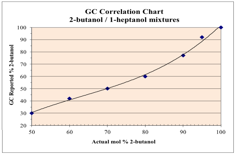
The calibration curve can then be used to correlate values reported by the GC instrument into true abundances. Imagine that a sample containing only 2-butanol and 1-heptanol is injected into the GC and reported by the instrument to be \(70\%\) 2-butanol. Using the calibration curve in Figure 2.85, a measured value of \(70\%\) 2-butanol (y-axis) correlates with an actual value of approximately \(87\) \(\text{mol}\%\) 2-butanol (x-axis). Therefore, a sample reported by the GC instrument to be \(70/30\%\) 2-butanol/1-heptanol, is actually closer to \(87/13\%\) 2-butanol/1-heptanol.
Due to the approximate nature of this method, percentage values should never be reported with more precision than the one's place, and probably the true error is on the order of \(\pm 5\%\).
Using Response Factors
Another method that can be used to translate the integration values given by the GC instrument into meaningful percentages is to use a response factor. A sample containing equimolar quantities of the compounds to be analyzed is injected into the GC and the peak areas are numerically translated into compound sensitivities.
This process will be demonstrated with a mixture containing only 2-butanol and 1-heptanol. Figure 2.86 shows the GC spectrum of a sample that contains equimolar quantities of 2-butanol and 1-heptanol.
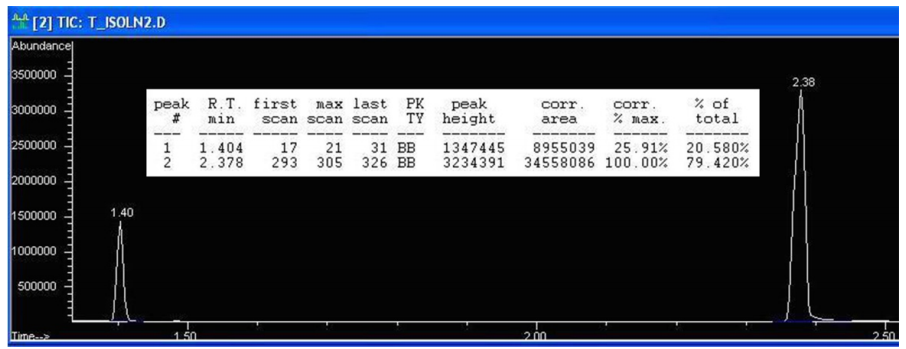
The peaks should have equal integrations because the compounds are present in equal molar amounts, but the peak at \(2.38 \: \text{min}\) (1-heptanol) is "counting" more than it should. In the quantitative report, the column with the header "corr.area" can be used, as this shows the calculated area of each peak. The ratio of these area counts (see calculation below) gives a value of 3.86, which means that 1-heptanol is detected 3.86 times "better" than 2-butanol in these mixtures.
\[\text{Ratio of corrected areas} = \frac{34558086 \: \text{area counts for 1-heptanol}}{8955039 \: \text{area counts for 2-butanol}} = 3.86\]
To use this response factor in correlating values reported by the GC instrument into true abundances, imagine that a sample containing only 2-butanol and 1-heptanol is reported by the GC to be \(30\%\) 1-heptanol (30 area counts of 1-heptanol for every 70 area counts of 2-butanol). As 1-heptanol is 3.86 times more responsive than 2-butanol, the true area counts would be more accurately represented as \(30/3.86 = 7.77\) area counts of 1-heptanol for every 70 area counts of 2-butanol.\(^{15}\)
\[\frac{30 \: \text{area counts for 1-heptanol}}{70 \: \text{area counts for 2-butanol}} \rightarrow \frac{30/3.86 \: \text{(1-heptanol)}}{70 \: \text{(2-butanol)}} = \frac{7.77 \: \text{(1-heptanol)}}{70 \: \text{(2-butanol)}}\]
These hypothetical (and yet more accurate) area counts can then be turned into percentages, as follows:
\[\% \: \text{1-heptanol} = \frac{7.77 \: \text{(1-heptanol)} \times 100\%}{70 + 7.77 \: \text{(total)}} = 10\% \: \text{1-heptanol, (meaning} \: 90\% \: \text{2-butanol)}\]
Therefore, a sample reported by the GC instrument to be \(70/30\%\) 2-butanol/1-heptanol, is actually closer to \(90/10\%\) 2-butanol/1-heptanol, which is a similar value to what could be found using a calibration curve.
\(^{15}\)These calculations could be done more succinctly and with more precision using the actual area counts for each peak, found in the "corr.area" column of a quantitative GC report.