14.1: An Introduction to NMR Spectroscopy
- Page ID
- 13933
\( \newcommand{\vecs}[1]{\overset { \scriptstyle \rightharpoonup} {\mathbf{#1}} } \)
\( \newcommand{\vecd}[1]{\overset{-\!-\!\rightharpoonup}{\vphantom{a}\smash {#1}}} \)
\( \newcommand{\id}{\mathrm{id}}\) \( \newcommand{\Span}{\mathrm{span}}\)
( \newcommand{\kernel}{\mathrm{null}\,}\) \( \newcommand{\range}{\mathrm{range}\,}\)
\( \newcommand{\RealPart}{\mathrm{Re}}\) \( \newcommand{\ImaginaryPart}{\mathrm{Im}}\)
\( \newcommand{\Argument}{\mathrm{Arg}}\) \( \newcommand{\norm}[1]{\| #1 \|}\)
\( \newcommand{\inner}[2]{\langle #1, #2 \rangle}\)
\( \newcommand{\Span}{\mathrm{span}}\)
\( \newcommand{\id}{\mathrm{id}}\)
\( \newcommand{\Span}{\mathrm{span}}\)
\( \newcommand{\kernel}{\mathrm{null}\,}\)
\( \newcommand{\range}{\mathrm{range}\,}\)
\( \newcommand{\RealPart}{\mathrm{Re}}\)
\( \newcommand{\ImaginaryPart}{\mathrm{Im}}\)
\( \newcommand{\Argument}{\mathrm{Arg}}\)
\( \newcommand{\norm}[1]{\| #1 \|}\)
\( \newcommand{\inner}[2]{\langle #1, #2 \rangle}\)
\( \newcommand{\Span}{\mathrm{span}}\) \( \newcommand{\AA}{\unicode[.8,0]{x212B}}\)
\( \newcommand{\vectorA}[1]{\vec{#1}} % arrow\)
\( \newcommand{\vectorAt}[1]{\vec{\text{#1}}} % arrow\)
\( \newcommand{\vectorB}[1]{\overset { \scriptstyle \rightharpoonup} {\mathbf{#1}} } \)
\( \newcommand{\vectorC}[1]{\textbf{#1}} \)
\( \newcommand{\vectorD}[1]{\overrightarrow{#1}} \)
\( \newcommand{\vectorDt}[1]{\overrightarrow{\text{#1}}} \)
\( \newcommand{\vectE}[1]{\overset{-\!-\!\rightharpoonup}{\vphantom{a}\smash{\mathbf {#1}}}} \)
\( \newcommand{\vecs}[1]{\overset { \scriptstyle \rightharpoonup} {\mathbf{#1}} } \)
\( \newcommand{\vecd}[1]{\overset{-\!-\!\rightharpoonup}{\vphantom{a}\smash {#1}}} \)
\(\newcommand{\avec}{\mathbf a}\) \(\newcommand{\bvec}{\mathbf b}\) \(\newcommand{\cvec}{\mathbf c}\) \(\newcommand{\dvec}{\mathbf d}\) \(\newcommand{\dtil}{\widetilde{\mathbf d}}\) \(\newcommand{\evec}{\mathbf e}\) \(\newcommand{\fvec}{\mathbf f}\) \(\newcommand{\nvec}{\mathbf n}\) \(\newcommand{\pvec}{\mathbf p}\) \(\newcommand{\qvec}{\mathbf q}\) \(\newcommand{\svec}{\mathbf s}\) \(\newcommand{\tvec}{\mathbf t}\) \(\newcommand{\uvec}{\mathbf u}\) \(\newcommand{\vvec}{\mathbf v}\) \(\newcommand{\wvec}{\mathbf w}\) \(\newcommand{\xvec}{\mathbf x}\) \(\newcommand{\yvec}{\mathbf y}\) \(\newcommand{\zvec}{\mathbf z}\) \(\newcommand{\rvec}{\mathbf r}\) \(\newcommand{\mvec}{\mathbf m}\) \(\newcommand{\zerovec}{\mathbf 0}\) \(\newcommand{\onevec}{\mathbf 1}\) \(\newcommand{\real}{\mathbb R}\) \(\newcommand{\twovec}[2]{\left[\begin{array}{r}#1 \\ #2 \end{array}\right]}\) \(\newcommand{\ctwovec}[2]{\left[\begin{array}{c}#1 \\ #2 \end{array}\right]}\) \(\newcommand{\threevec}[3]{\left[\begin{array}{r}#1 \\ #2 \\ #3 \end{array}\right]}\) \(\newcommand{\cthreevec}[3]{\left[\begin{array}{c}#1 \\ #2 \\ #3 \end{array}\right]}\) \(\newcommand{\fourvec}[4]{\left[\begin{array}{r}#1 \\ #2 \\ #3 \\ #4 \end{array}\right]}\) \(\newcommand{\cfourvec}[4]{\left[\begin{array}{c}#1 \\ #2 \\ #3 \\ #4 \end{array}\right]}\) \(\newcommand{\fivevec}[5]{\left[\begin{array}{r}#1 \\ #2 \\ #3 \\ #4 \\ #5 \\ \end{array}\right]}\) \(\newcommand{\cfivevec}[5]{\left[\begin{array}{c}#1 \\ #2 \\ #3 \\ #4 \\ #5 \\ \end{array}\right]}\) \(\newcommand{\mattwo}[4]{\left[\begin{array}{rr}#1 \amp #2 \\ #3 \amp #4 \\ \end{array}\right]}\) \(\newcommand{\laspan}[1]{\text{Span}\{#1\}}\) \(\newcommand{\bcal}{\cal B}\) \(\newcommand{\ccal}{\cal C}\) \(\newcommand{\scal}{\cal S}\) \(\newcommand{\wcal}{\cal W}\) \(\newcommand{\ecal}{\cal E}\) \(\newcommand{\coords}[2]{\left\{#1\right\}_{#2}}\) \(\newcommand{\gray}[1]{\color{gray}{#1}}\) \(\newcommand{\lgray}[1]{\color{lightgray}{#1}}\) \(\newcommand{\rank}{\operatorname{rank}}\) \(\newcommand{\row}{\text{Row}}\) \(\newcommand{\col}{\text{Col}}\) \(\renewcommand{\row}{\text{Row}}\) \(\newcommand{\nul}{\text{Nul}}\) \(\newcommand{\var}{\text{Var}}\) \(\newcommand{\corr}{\text{corr}}\) \(\newcommand{\len}[1]{\left|#1\right|}\) \(\newcommand{\bbar}{\overline{\bvec}}\) \(\newcommand{\bhat}{\widehat{\bvec}}\) \(\newcommand{\bperp}{\bvec^\perp}\) \(\newcommand{\xhat}{\widehat{\xvec}}\) \(\newcommand{\vhat}{\widehat{\vvec}}\) \(\newcommand{\uhat}{\widehat{\uvec}}\) \(\newcommand{\what}{\widehat{\wvec}}\) \(\newcommand{\Sighat}{\widehat{\Sigma}}\) \(\newcommand{\lt}{<}\) \(\newcommand{\gt}{>}\) \(\newcommand{\amp}{&}\) \(\definecolor{fillinmathshade}{gray}{0.9}\)5.1A: NMR-active nuclei
The basis for nuclear magnetic resonance is the observation that many atomic nuclei spin about an axis and generate their own magnetic field, or magnetic moment. For reasons that are outside the scope of this text, only those nuclei with an odd number of protons and/or neutrons have a magnetic moment. Fortunately for chemists, several common nuclei, including hydrogen (1H), the 13C isotope of carbon, the 19F isotope of fluorine, and the 31P isotope of phosphorus, all have magnetic moments and therefore can be observed by NMR – they are, in other words, NMR-active. Other nuclei - such as the common 12C and 16O isotopes of carbon and oxygen - do not have magnetic moments, and are essentially invisible in NMR. Other nuclei such as deuterium (2H) and nitrogen (14N) have magnetic moments and are NMR-active, but the nature of their magnetic moments is such that these nuclei are more difficult to analyze by NMR. In practice it is 1H, 13C, 19F, and 31P that are most often observed by NMR spectroscopy. In this chapter, we will develop our understanding of the principles behind NMR spectroscopy by focusing our attention first on the detection of protons in 1H-NMR experiments (in discussion about NMR, the terms 'hydrogen' and 'proton' are used interchangeably). Much of what we learn, however, will also apply to the detection and analysis of other NMR-active nuclei, and later in the chapter we will shift our attention to NMR experiments involving 13C and 31P atoms.
5.1B: Nuclear precession, spin states, and the resonance condition
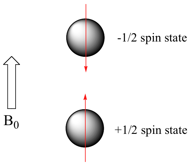
When a sample of an organic compound is sitting in a flask on a laboratory benchtop, the magnetic moments of its hydrogen atoms are randomly oriented. When the same sample is placed within the field of a very strong magnet in an NMR instrument (this field is referred to by NMR spectroscopists as the applied field, abbreviated B0 ) each hydrogen will assume one of two possible spin states. In what is referred to as the +½ spin state, the hydrogen's magnetic moment is aligned with the direction of B0, while in the -½ spin state it is aligned opposed to the direction of B0.

Because the +½ spin state is slightly lower in energy, in a large population of organic molecules slightly more than half of the hydrogen atoms will occupy this state, while slightly less than half will occupy the –½ state. The difference in energy between the two spin states increases with increasing strength of B0.This last statement is in italics because it is one of the key ideas in NMR spectroscopy, as we shall soon see.
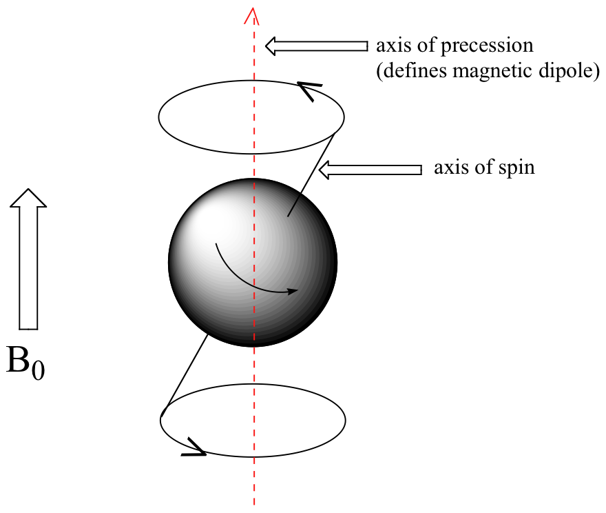
At this point, we need to look a little more closely at how a proton spins in an applied magnetic field. You may recall playing with spinning tops as a child. When a top slows down a little and the spin axis is no longer completely vertical, it begins to exhibit precessional motion, as the spin axis rotates slowly around the vertical. In the same way, hydrogen atoms spinning in an applied magnetic field also exhibit precessional motion about a vertical axis. It is this axis (which is either parallel or antiparallel to B0) that defines the proton’s magnetic moment. In the figure below, the proton is in the +1/2 spin state.

The frequency of precession (also called the Larmour frequency, abbreviated ωL) is simply the number of times per second that the proton precesses in a complete circle. A proton`s precessional frequency increases with the strength of B0.
If a proton that is precessing in an applied magnetic field is exposed to electromagnetic radiation of a frequency ν that matches its precessional frequency ωL, we have a condition called resonance. In the resonance condition, a proton in the lower-energy +½ spin state (aligned with B0) will transition (flip) to the higher energy –½ spin state (opposed to B0). In doing so, it will absorb radiation at this resonance frequency ν = ωL. This frequency, as you might have already guessed, corresponds to the energy difference between the proton’s two spin states. With the strong magnetic fields generated by the superconducting magnets used in modern NMR instruments, the resonance frequency for protons falls within the radio-wave range, anywhere from 100 MHz to 800 MHz depending on the strength of the magnet.

