11.3.2: Correlation Diagrams

Splitting of Terms in an Octahedral Field

Figure \(\PageIndex{1}\): Octahedral field term splitting

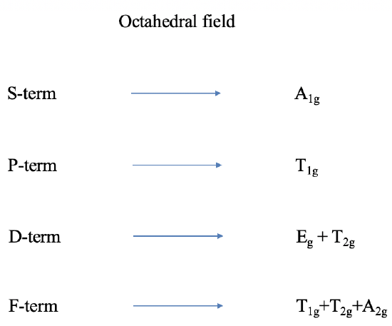
Thus far we have only considered free ion terms, which means terms without the presence of a ligand field. Let us think next about the influence of an octahedral field on a term. Terms are wavefunctions, just like orbitals, and therefore they behave like orbitals in a ligand field. For example, the \(d\)-orbitals split into \(t_{2g}\)and \(e_g\) orbitals in an octahedral ligand field. A \(D\)-term behaves similarly. It splits into \(T_{2g}\) and \(E_g\) terms (note the capital letters that describe term, and the lower-case letters that describe orbitals!). \The \(p\)-orbitals are triple-degenerate, having \(T_{1g}\) symmetry in the \(O_h\) (octahedral) point group, and do not split in energy: they give the \(t_{1g}\) orbitals under an octahedral field. Similarly, the \(P\)-terms have the same symmetry and also do not split. The \(P\)-term becomes a \(T_{1g}\) term in an octahedral field.

Following analogous arguments, \(S\) terms become \(A_{1g}\) terms. \(F\) terms do split in energy like \(f\)-orbitals and become \(T_{1g}\), \(T_{2g}\), and \(A_{2g}\) terms. Overall, the presence of the octahedral field increases the number of terms from four to seven (Figure \(\PageIndex{1}\)). It is easy to see that the ligand field leads to many states, and many potential electron transitions. Thus, we would expect quite complicated spectra. For other ligand fields, the terms also behave analogously to orbitals. For, instance in a tetrahedral field D-terms split into E and T₂ terms, and so forth.

Term Splitting for octahedral d² metal complexes

Now let us think about how the term energies of our free d²-ion changes when placed in an octahedral ligand field, depending on the ligand field strength. We can express this by a correlation diagram (Figure \(\PageIndex{2}\)). In a correlation diagram, we plot the energies of the terms relative to the field strength.

Figure \(\PageIndex{2}\): Correlation diagram

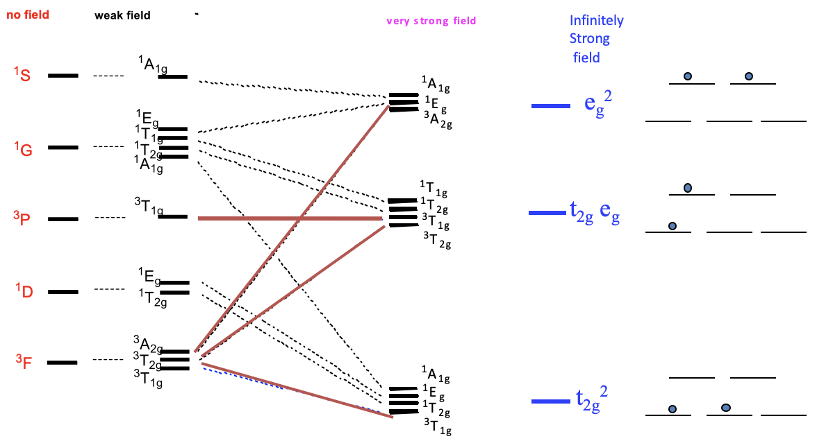
On the left side we plot the terms without any field according to their energies. In the case of a d² ion, the energies are

\[\ce{^{3}F < ^{1}D < ^{3}P < ^{1}G < ^{1}S}. \nonumber\]

Next, we plot the relative energies in a weak octahedral ligand field, and label the terms according to their symmetry. We can see that the D, F, and G terms split in energy, while the S and P terms do not. Because of the weak field, energy differences are very small. Now let us increase the ligand field strength continuously, until we have reached a very strong ligand field. We see that some of the terms move up in energy, while other terms move down as the ligand field increases. For example, two of the three terms resulting from the F-terms increase in energy while one decreases. It is also possible that a term does not change its energy. For example, the ³T_1g term from the ³P term does not change its energy. In very strong ligand field there are three groups of terms that have similar energy. In the hypothetical case of an infinitely strong ligand field, the terms that belong to a particular group become identical in energy. In this case, there are only three states for the electrons possible. The field is considered so strong that the energy associated with electron-electron interactions become negligible compared to the energy of the field. The electrons behave as though there were no electron-electron interactions. Therefore, we can call the lowest energy state the t_2g² state. It is equivalent to the state of the two electrons being in the t_2g orbitals. The second state is called the t_2ge_g state. It is equivalent to the state of one electron being in the t_2g and one electron being in the e_g orbitals. The third state is called the e_g² state, which is equivalent to the state with both electrons in the e_g²-orbitals.