8.1.4.2: Frost Diagrams show how stable element's redox states are relative to the free element

Frost diagrams show how stable an element's redox states are relative to the free element

Frost diagrams represent how stable an element's redox states are relative to the free element. In a Frost diagram, a proxy for the free energy relative to that of the free element (oxidation state zero) is plotted as a function of oxidation state. To avoid ambiguity, sometimes the points are labeled with the identity of the chemical species involved.

The proxy used in place of the free energy is \(NE^{\circ}\), sometimes expressed as \(nE^{\circ}\). On this page \(N\) will be used in place of \(n\) to avoid confusion with the common use of \(n\) in redox chemistry to denote the number of electrons involved in individual oxidation or reduction reaction steps.

In Frost diagrams the quantity \(NE^{\circ}\) is used since it is proportional to the standard free energy change for conversion of the free element to that oxidation state.

In \(NE^{\circ}\)

• \(N\) is the oxidation state.
• \(\sf{E^{\circ}}\) is the standard reduction potential associated with interconversion between the free element and that oxidation state.

For a proof that \(NE^{\circ}\) is proportional to the free energy of an element's oxidation state and more information on how \(NE^{\circ}\) may be calculated, see Note \(\PageIndex{1}\) at the end of this page.

Frost diagrams allow for rapid estimation of the relative stability of elements' redox states.

Because Frost diagrams directly show oxidation states' relative stabilities, they enable the rapid assessment of the following:

1. The relative stability of an element's oxidation states under a given set of conditions. Since \(NE^{\circ}\) is a measure of thermodynamic stability, the lower its value the more stable the state. Moreover, since \(NE^{\circ}\) measures stability relative to the free element, negative values of \(NE^{\circ}\) indicate that a state is more stable than the element, while positive values indicate that the state is less stable.

Consider the Frost diagram for copper at pH 0 shown in Figure \(\PageIndex{1}\).

Figure \(\PageIndex{1}\). Frost diagram for copper in aqueous acid. (CC BY-SA 4.0 International; Stephen Contakes)

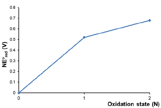
As can be seen in Figure \(\sf{\PageIndex{1}}\), Cu⁺ and Cu²⁺ are both higher in free energy (\(\propto NE^{\circ}\)) than free Cu. This is consistent with copper's status as a noble metal that can only be dissolved in acid with the aid of oxidizing agents like O₂, H₂O₂, or NO₃^- (e.g., as in HNO₃).

The acidic Frost diagram of Nickel shown in Figure \(\PageIndex{2}\) provides an example of a metal which dissolves in acid under otherwise nonoxidizing conditions (i.e., without the aid of oxidants like O₂ or H₂O₂).

Figure \(\PageIndex{2}\). Frost diagram for nickel in aqueous acid. (CC BY-SA 4.0 International; Stephen Contakes)

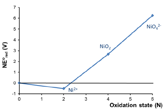
In this case the diagram shows that the Ni²⁺ oxidation state is lower in free energy than the free element, indicating that Ni spontaneously dissolves in acid to give Ni²⁺. The diagram also reveals that higher nickel oxidation states (+4 and +6) are known but unstable with respect to both Ni²⁺ and free nickel.

Example \(\PageIndex{1}\). Interpreting a Frost Diagram

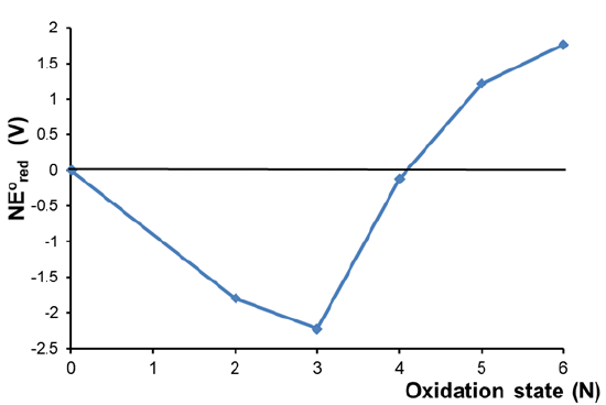
Consider the Frost diagram of Cr in acid shown in Figure \(\PageIndex{3}\). What can be determined about the relative stability of chromium's oxidation states in acid?

Figure \(\PageIndex{3}\). Frost diagram for Cr in acidic solution. This work by Stephen Contakes is licensed under a Creative Commons Attribution 4.0 International License.

Solution

A cursory glance at the diagram reveals that

• The +3 oxidation state is the most stable since it has the lowest \(NE^{\circ}\).
• The +2, +3, and +4 oxidation states are all more stable than the free element while the +5 and +6 oxidaton states are less stable.
• The diagram also reveals information about the susceptibility of the chromium species to undergo disproportionation and comproportionation reactions. For details see example 2.

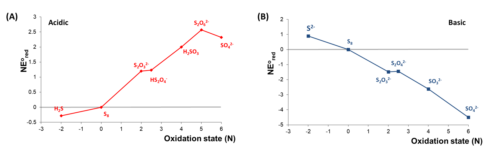
2. The redox behavior of an element under different conditions. Consider the Frost diagrams of sulfur at pH 0 and 14 shown in Figure \(\PageIndex{4}\).

Figure \(\PageIndex{4}\). Frost diagrams for sulfur at pH 0 and 14. This work by Stephen Contakes is licensed under a Creative Commons Attribution 4.0 International License.

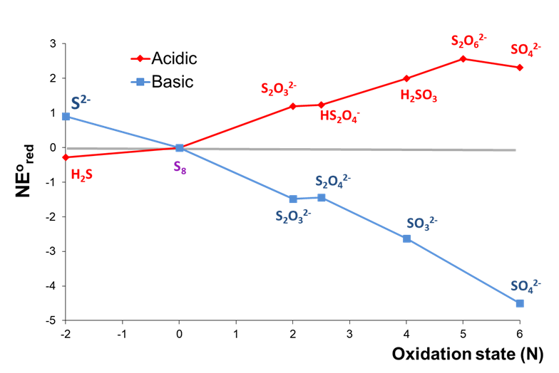
As can be seen in Figure \(\PageIndex{4}\), the relative stabilities of high and low sulfur oxidation states are roughly inverted between acidic and basic conditions. Under basic conditions, the oxidized forms of sulfur are all more stable than the free element, with sulfate most stable overall. In contrast, H₂S is the most stable form of sulfur under acidic conditions, while all the oxidized forms of sulfur are less stable than the free element.

3. Comparison of the redox behavior of a series of elements. Consider the pH 0 Frost diagrams of the group 6 elements shown in Figure \(\PageIndex{5}\).

Figure \(\PageIndex{5}\). Frost diagrams for the group 6 elements at pH 0. This work by Stephen Contakes is licensed under a Creative Commons Attribution 4.0 International License.

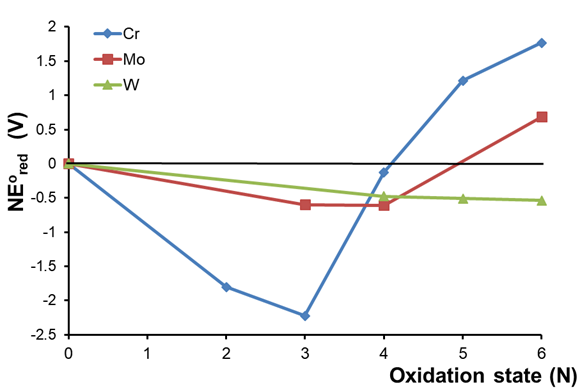
Several trends may be noted from the data in Figure \(\PageIndex{5}\). First, on moving down the group from Cr to W, there is an increasing preference for higher oxidation states, with the most stable forms being Cr⁴⁺, Mo⁴⁺, and W⁶⁺. Second, the coincidentally low stabilization of Cr⁴⁺ aside, the stabilization or destabilization of oxidation states relative to the free element decreases down a group - i.e., Cr⁴⁺ is stabilized relative to Cr more so than Mo⁴⁺ is relative to Mo, and W⁶⁺ is stabilized relative to W even less so.

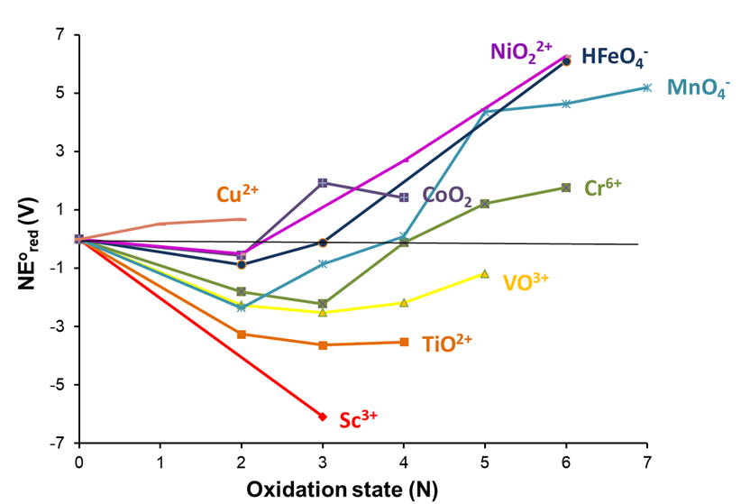
One of the most striking examples of the utility of Frost diagrams for comparing the empirical redox behavior of a series of elements involves the first row transition elements, the pH 0 Frost diagrams for which are shown in Figure \(\PageIndex{6}\).^2,3 A number of trends may be noted. For example, as in the case of the group 6 elements, a shift in the most stable oxidation state may be observed, with Sc through Cr exhibiting a preference for the +3 oxidation state and Mn through Cu the +2 oxidation state. The diagram also shows that Sc through Mn lose all their valence electrons to form d⁰ species, while similar species have not been observed for later members of the series (although an iron(VII) complex has been isolated⁴ and iron's heavier cogeners, Ru and Os, do form d⁰ species, RuO₄ and OsO₄).

Figure \(\PageIndex{6}\). Frost diagrams for the first transition series at pH 0. This work by Stephen Contakes is licensed under a Creative Commons Attribution 4.0 International License.

4. Whether a redox state is unstable towards disproportionation may be determined from the relative positions of that state and the states on either side of it on the diagram.⁵ Remember that in disproportionation a species reacts with itself to produce two or more stable products. For example, NO can in principle undergo disproportionation in aqueous acid to give nitrate and N₂.

\[\sf{ 10~NO~+~2H_2O \rightarrow 3~N_2 + 4~NO_3^- + 4H^+ } \nonumber \]

A Frost diagram can be used to determine when a redox state is unstable with respect to such disproportionation because the slope of a line between any two points is equal to the standard reduction potential interconverting the species involved. This means that if a line is drawn between any two redox states then any states above the line will be unstable towards disproportionation to those states. This is because in that case the potential for the reduction half reaction in the disproportionation will be more positive than the potential for the oxidation half reaction, rendering the overall reaction potential positive and so spontaneous. For proof of a specific example see Exercise 1.

To see how a disproportionation analysis may be performed using a Frost diagram, it can be helpful to examine the pH 0 Frost diagram for Cr more carefully. In this case the instability of Cr⁴⁺ and Cr⁵⁺ towards disproportionation may be revealed by placing a tie line drawn between the Cr³⁺ and Cr⁶⁺ states, as shown in Figure \(\PageIndex{7a}\).

Figure \(\PageIndex{7}\). (a) Frost diagram for Cr in acidic solution showing that the Cr⁴⁺ and Cr⁵⁺ states lie above a tie-line between the Cr³⁺ and Cr⁶⁺ states. (b) In the case of Cr⁴⁺, disproportionation is favored because the Cr^4/3+ potential (slope of the green tie-line connecting the Cr⁴⁺ and Cr³⁺ states) is larger than the Cr^6/4+ potential (slope of the pink tie-line connecting Cr⁶⁺ and Cr⁴⁺). This work by Stephen Contakes is licensed under a Creative Commons Attribution 4.0 International License.

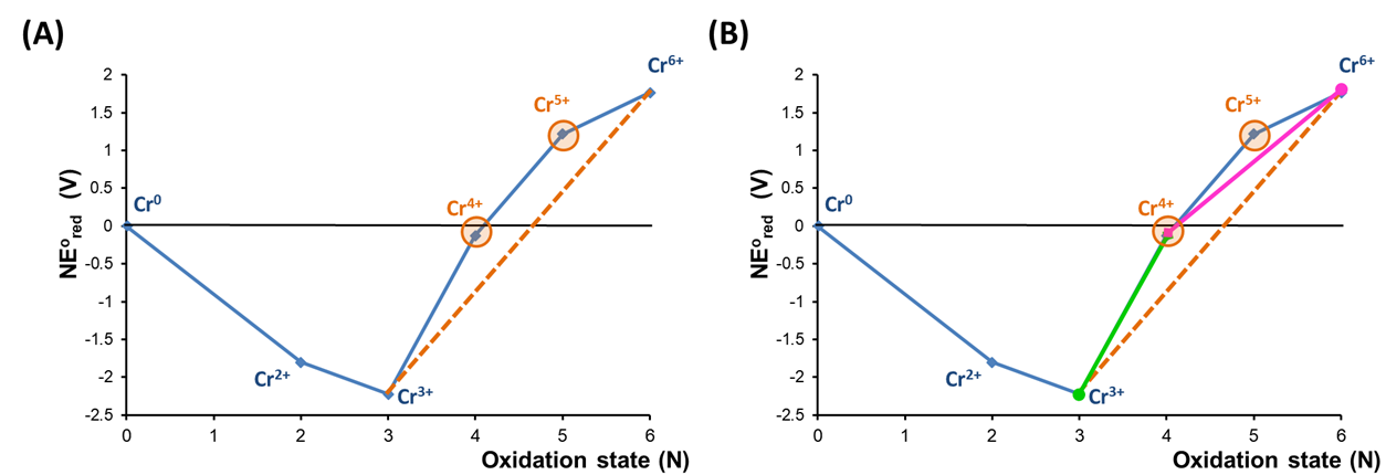
As shown in Figure \(\PageIndex{7a}\), the Cr⁴⁺ and Cr⁵⁺ states are unstable towards disproportionation because they lie above a tie-line between the Cr³⁺ and Cr⁶⁺ states. This is because the potential for Cr⁴⁺ reduction to Cr³⁺, represented by the tie-line connecting those species in Figure \(\PageIndex{7b}\), is larger than the potential for Cr⁶⁺ reduction to Cr⁴⁺, as indicated by the lower slope of the tie-line connecting Cr⁶⁺ and Cr⁴⁺.

Sometimes states which are unstable towards disproportionation correspond to concave down points on the Frost diagram. However, as this is not always the case, a systematic approach for finding metastable redox states is recommended. An example of such an approach is given in Example \(\PageIndex{2}\).

Example \(\PageIndex{2}\). Systematic identification of Mn redox states that are unstable towards disproportionation in acid.

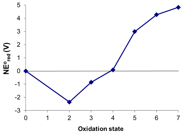
Consider the Frost diagram of Mn in acid shown in Figure \(\PageIndex{8}\). Which, if any, of manganese's oxidation states are unstable towards disproportionation at pH 0?

Figure \(\PageIndex{8}\). Frost diagram for Mn at pH 0. This work by Stephen Contakes is licensed under a Creative Commons Attribution 4.0 International License.

Solution

States that are unstable towards disproportionation may be identified by drawing all the possible tie-lines between nonadjacent states spanning the lowest and highest oxidation states in the diagram, which in this case are Mn⁰ and Mn⁷. The possible permutations beginning with Mn⁰ are given below

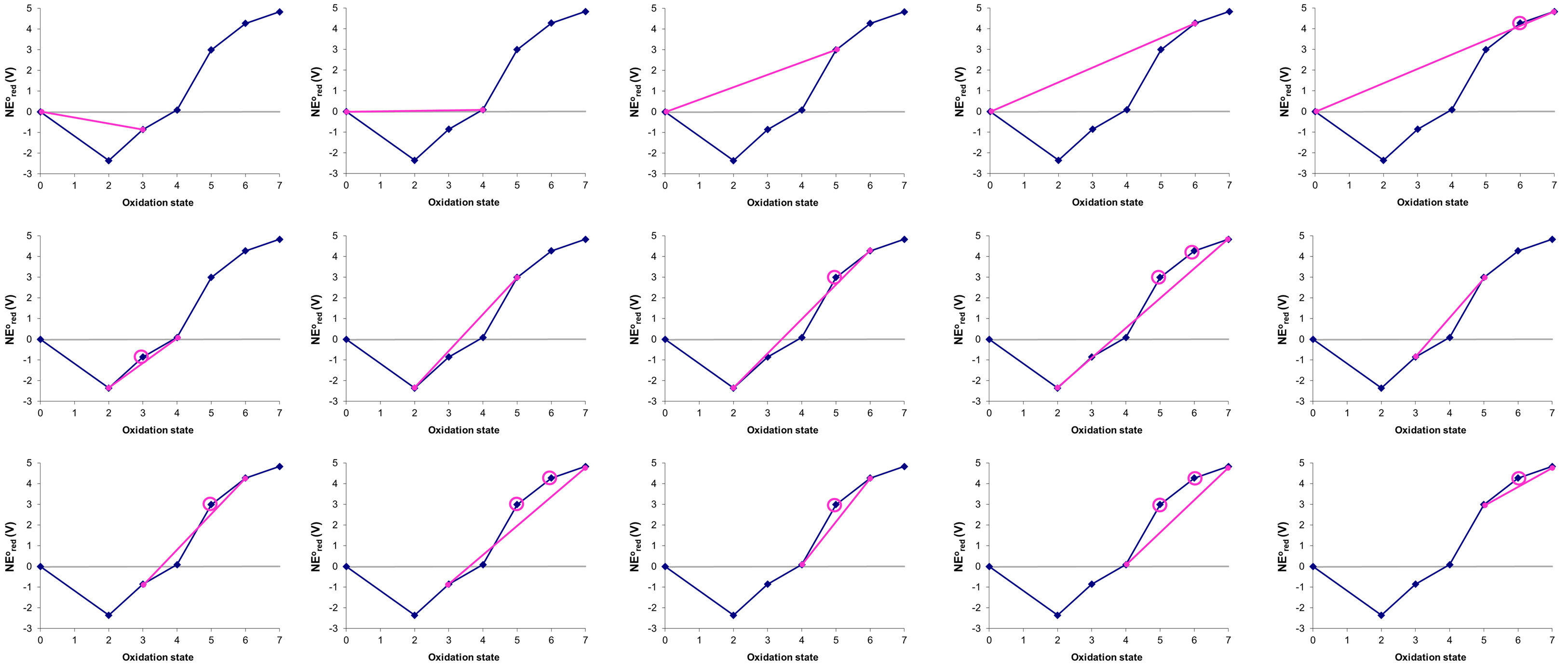
In the figure above the states that are thermodynamically unstable towards disproportionation (circled) are +3, +5, and +6.

The figure above by Stephen Contakes is licensed under a Creative Commons Attribution 4.0 International License.

4. Whether two species are unstable towards comproportionation may be assessed from the relative positions of the two species and all intervening species on the diagram. In comproportionation, two related species react to give a more stable product. For example, NO and hydrazinium ion can in principle undergo comproportionation in aqueous acid to give N₂.

\[\sf{2~NO~~+~~N_2H_5^+}~ \rightarrow \sf{2~N_2~~+~~2~H_2O~~+~~H^+ } \nonumber \]

A Frost diagram may be used to determine when two species are thermodynamically favored to undergo comproportionation. Draw a line between the two species on the diagram. If there are states below the line then the two species are unstable towards forming those states by comproportionation. Again, it can be helpful to examine the acidic condition Frost diagram for Cr to see how this works. In this case consider a tie line drawn between the Cr⁴⁺ and Cr²⁺ states, as shown in Figure \(\PageIndex{9a}\).

Figure \(\PageIndex{9}\). (a) Frost diagram for Cr in acidic solution showing that the Cr³⁺ redox state lies below a tie-line between the Cr²⁺ and Cr⁴⁺ states. (b) The slope of the green line connecting the Cr²⁺ and Cr³⁺ states is less than that of the pink line connecting the Cr³⁺ and Cr⁴⁺ states. This work by Stephen Contakes is licensed under a Creative Commons Attribution 4.0 International License.

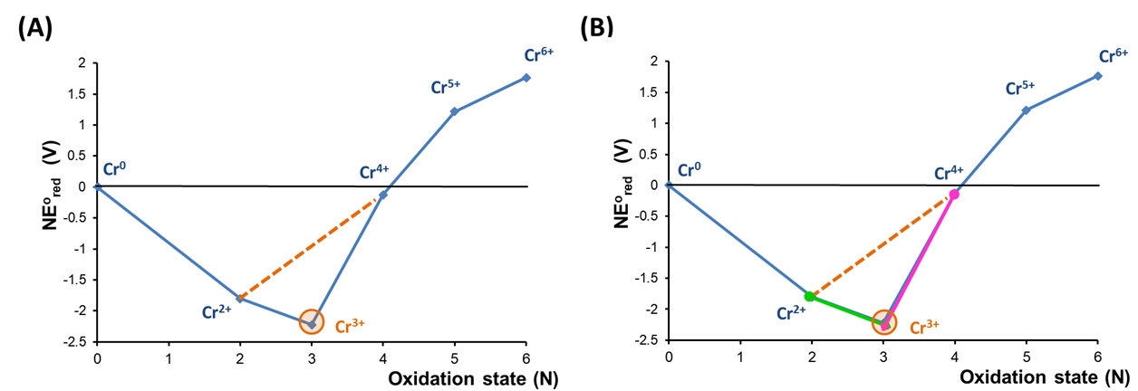
As shown in Figure \(\PageIndex{9a}\), a mixture of Cr²⁺ and Cr⁴⁺ is unstable towards comproportionation because on the Frost diagram Cr³⁺ lies below the tie-line between Cr²⁺ and Cr⁴⁺. This shows that the standard potential for reduction of Cr³⁺ to Cr²⁺ (equal to the slope of the line connecting those states) is less than that for the reduction of Cr⁴⁺ to Cr³⁺ (again, equal to that of the line connecting the states), in consequence of which the potential for comproportionation will be positive.

The analysis of a Frost diagram for all favorable comproportionations is similar to the analysis used to detect species that are unstable towards disproportionation. The products of thermodynamically favored comproportionations are sometimes concave up points but since this is not always the case a systematic approach should be used. An example is given in Example \(\PageIndex{3}\).

Example \(\PageIndex{3}\). Systematic identification of pairs of Mn redox states that are unstable towards comproportionation in acid.

Consider the Frost diagram of Mn at pH 0 in Figure \(\PageIndex{8}\) of Example \(\PageIndex{2}\), which for convenience is reproduced below. Which, if any, pairs of manganese species are unstable towards comproportionation under these conditions and what products could they form?

Solution

The possible tie-lines were already identified in Exercise \(\PageIndex{2}\).

Figure above: the lower energy comproportionation products that species form are circled in green. The comproportionations identified involve the following pairs of oxidation states:

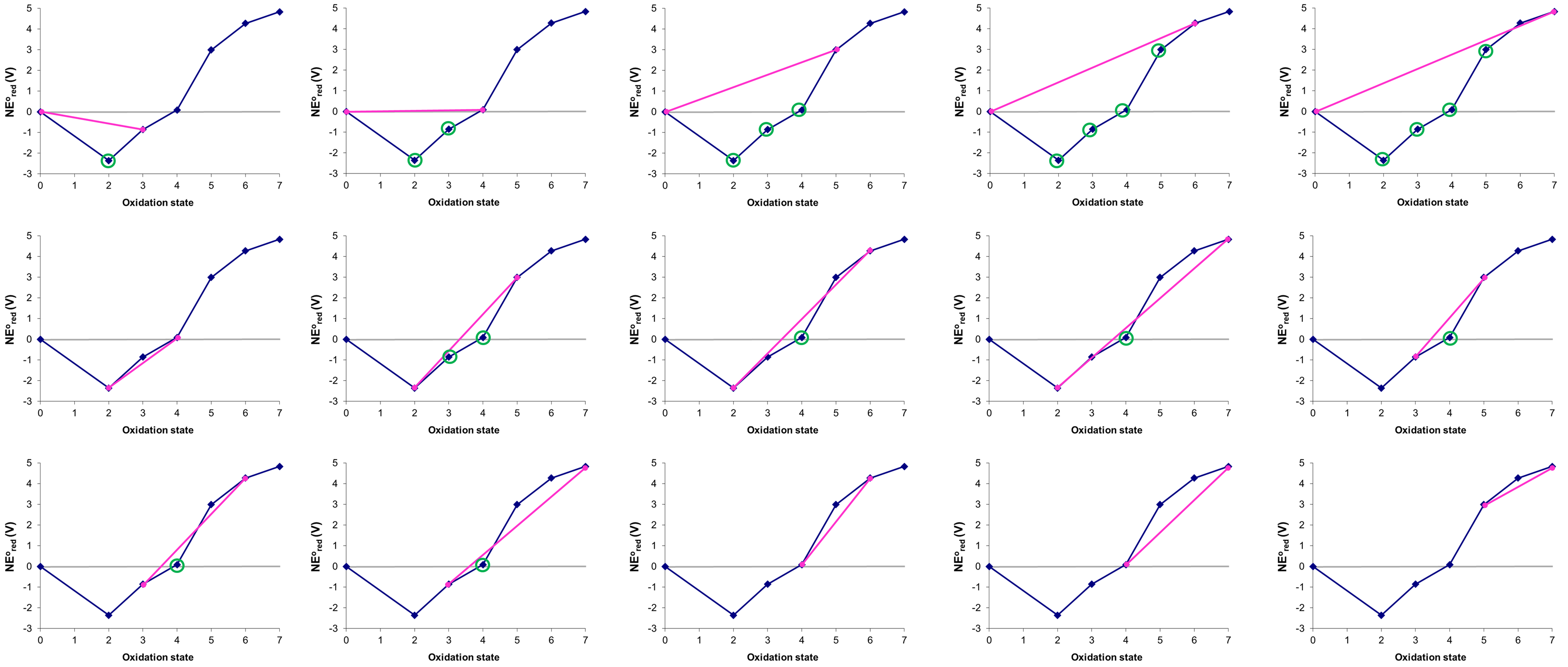
• 0 and +3 \(\rightarrow\) +2
• 0 and +4 \(\rightarrow\) +2 or +3
• 0 and +5 \(\rightarrow\) +2 or +3 or +4
• 0 and +6 \(\rightarrow\) +2 or +3 or +4 or +5
• 0 and +7 \(\rightarrow\) +2 or +3 or +4 or +5
• +2 and +5 \(\rightarrow\) +3 or +4
• +2 and +6 \(\rightarrow\) +4
• +2 and +7 \(\rightarrow\) +4
• +3 and +5 \(\rightarrow\) +4
• +3 and +6 \(\rightarrow\) +4
• +3 and +7 \(\rightarrow\) +4

The figures in this problem are by Stephen Contakes and licensed under a Creative Commons Attribution 4.0 International License.

Additional analysis is needed to determined the thermodynamic product of many comproportionation reactions - but fortunately such an analysis is not necessary to understand the descriptive chemistry of the elements.

This list of possible comproportionation reactions identified in Example \(\PageIndex{3}\) raises several interesting questions:

1. When more than one comproportionation product is possible, which one(s) will be formed?

In this case the answer is that all species can be formed in thermodynamically favored comproportionation reactions. However, the system still only possesses one state of lowest free energy. For example, depending on the stoichiometry of the reactants, the lowest energy products that can be formed from a mixture of Mn⁰ and Mn^VII might be a mixture of Mn^II and Mn^IV. The identification of this state in a given case is complicated and involves minimizing the system energy subject to the constraints of a mass and charge balance. Fortunately, such an analysis is not needed to make sense of the chemistry of the elements.

What should be noted is that if a comproportionation product can itself undergo a comproportionation reaction with one or more reactants, then that reaction can take place in solution. For instance, if the case of the comproportionation between Mn⁰ and Mn^IV produces Mn^III, then that Mn^III can undergo an additional comproportionation reaction with Mn⁰ to give Mn^II.

2. What happens if a species formed by comproportionation is susceptible to disproportionation?

If the conditions allow, then that species will undergo disproportionation. Again, thermodynamic measures like those shown on Frost diagrams describe what can happen, not what will occur under a given set of conditions.

Exercises

Exercise \(\PageIndex{1}\)

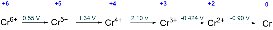
Using the simplified Latimer diagram for Cr in aqueous acid, reproduced below, verify that the disproportionation of Cr⁴⁺ to Cr³⁺ and Cr⁶⁺ is thermodynamically spontaneous.

Answer

The disproportionation of Cr⁴⁺ to Cr³⁺ and Cr⁶⁺ is the sum of two processes:

\[\sf{ Cr^{4+} reduction:~~~~~~~Cr^{4+} + e^- \rightarrow Cr^{3+}~~~~~~~~~~~~~~~E^{\circ}_{Cr^{4/3+}}=~2.10~V } \nonumber \]

\[\sf{ Cr^{4+} oxidation:~~~Cr^{4+} \rightarrow Cr^{6+}~+~2e^- ~~~~~~~E^{\circ}=-E^{\circ}_{Cr^{6/4+}} } \nonumber \]

---

\[\sf{Sum:~~3Cr^{4+} + \rightarrow Cr^{6+}~+~2Cr^{3+} ~~~~~~~~~~~~E^{\circ}_{\sf{disproportionation}}=E^{\circ}_{Cr^{4/3+}}~~-~~E^{\circ}_{Cr^{6/4+}} } \nonumber \]

The value of \(E^{\circ}_{Cr^{6/4+}}\) is just the sum of the Cr^6/5+ and Cr^5/4+ reduction potentials (+0.55 V + 1.34 V) or +1.89 V. Consequently,

\[ E^{\circ}_{\sf{disproportionation}} = E^{\circ}_{\sf{Cr^{4/3+}}}~~~~~E^{\circ}_{Cr^{6/4+}}~\sf{=~2.10~V~~-~1.89~V~~=~~+0.21~V} \nonumber \]

which is spontaneous.

Exercise \(\PageIndex{2}\)

Using the simplified Latimer diagram for Cr in aqueous acid, reproduced below, verify that the comproportionation of Cr²⁺ and Cr⁴⁺ to Cr³⁺ is thermodynamically spontaneous.

Answer

The comproportionation of Cr²⁺ and Cr⁴⁺ to Cr³⁺ is the sum of two processes:

\[\sf{ Cr^{4+} reduction:~~~~~~~Cr^{4+} + e^- \rightarrow Cr^{3+}~~~~~~~~~~~~~~~E^{\circ}_{Cr^{4/3+}}~=~+2.10~V } \nonumber \]

\[\sf{ Cr^{2+} oxidation:~~~Cr^{2+} \rightarrow Cr^{3+}~+~e^- ~~~~~~~E^{\circ}=-E^{\circ}_{Cr^{3/2+}}~= -(-0.424~V)~=~=~+0.424~V} \nonumber \]

---

\[\sf{Sum:~~Cr^{2+} + Cr^{4+} \rightarrow 2Cr^{3+} ~~~~~~~~~~~~E^{\circ}_{\sf{comproportionation}}~=~+2.10~V~~+~~0.424~V~~=~~+2.524~V} \nonumber \]

Since \(E^{\circ}_{\sf{comproportionation}}\) is positive, the comproportionation is spontaneous.

Exercise \(\PageIndex{3}\). Identifying thermodynamically favored comproportionation and disproportionation reactions.

The Frost diagrams for acidic and basic solutions of sulfur are given below.

a. Identify any species that are unstable towards disproportionation under acidic or basic conditions.

b. Identify any species that can be formed by comproportionation under acidic or basic conditions.

Answer

The species that are unstable towards disproportionation and comproportionation may be identified by constructing tie-lines between nonadjacent redox states and identifying any that fall above and below these lines. Species that are unstable to disproportionation will lie above a line; those that will be formed by comproportionation will lie below a line. Note that some species may be both capable of being formed by comproportionation and thermodynamically susceptible to disproportionation.

The possible tie-lines for acidic conditions are as follows:

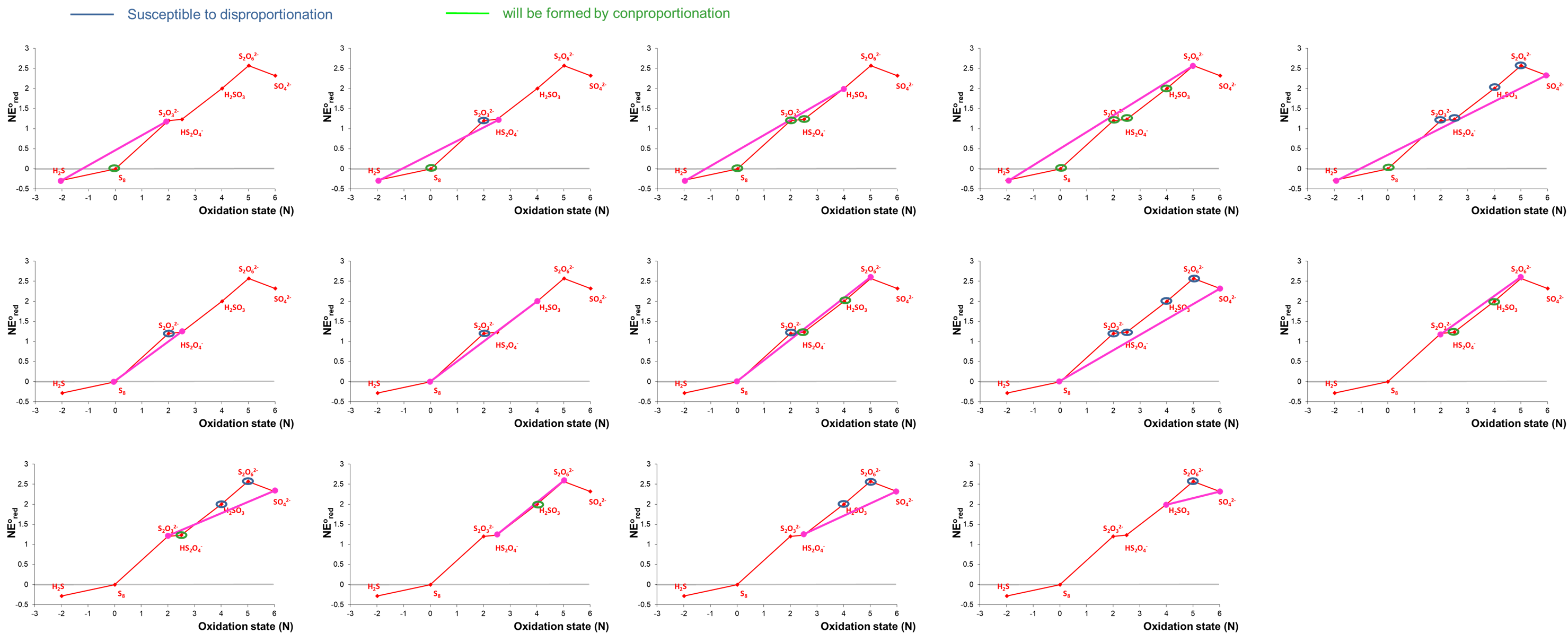
Notice that in some cases it can be difficult to tell whether a point lies above or below a tie-line based on inspection alone. In these cases the relevant redox potential should be calculated to determine whether disproportionation or comproportionation is thermodynamically favored or even if the process is free energy neutral.

The possibilities for basic conditions are left as an exercise for the reader. To check your work the species that are susceptible to disproportionation and those which can be formed by comproportionation are summarized below.

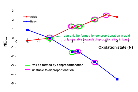
The figures in this problem are by Stephen Contakes and licensed under a Creative Commons Attribution 4.0 International License.

Appendix

Note \(\PageIndex{1}\). Construction of a Frost Diagram.

Since Frost diagrams use \(NE^{\circ}\) as a proxy for oxidation free energy, the construction of a Frost diagram is a matter of calculating \(NE^{\circ}\) for each oxidation state, where \(E^{\circ}\) is the standard potential for the formation of that oxidation state (O.S.) from the free element. To see why this quantity is a useful proxy for oxidation state free energy, it is helpful to recognize that the oxidation state, N, is formally equal to the number of electrons that are removed from the free element when the oxidation state is formed. From this perspective the formation of negative oxidation states by adding electrons to the free element may be thought of as involving the removal of a negative number of electrons.

The free energy for formation of each oxidation state is determined as follows:

1. For free elements the free energy of formation, \(E^{\circ}\), and consequently \(NE^{\circ}\), are all by definition zero.

2. Negative oxidation states are formed by reduction of the free element

\[E + ne^- \rightarrow E^{O.S.}~~~~~~~~~E^{\circ}=E^{\circ}_{red} \nonumber \]

so that

\[ \Delta G^{\circ} = -n F E^{\circ}_{red} \nonumber \]

in which \(F\) is the Faraday constant.

In this case the oxidation state, \(N\), is equal to \(-n\) and the expression above becomes

\[ \Delta G^{\circ}_{red} = F \times (NE^{\circ}) \nonumber \]

from which it can also be seen why \(NE^{\circ}\) is a useful proxy for free energy. It is proportional to \(\Delta G^{\circ}\):

\[NE^{\circ}= \dfrac{1}{F} \Delta G^{\circ}_{red} \nonumber \]

3. Positive oxidation states are formed by oxidation of the element:

\[E \rightarrow E^{O.S.} + ne^-~~~~~~~~~E^{\circ}_{ox} = E^{\circ}=-E^{\circ}_{red} \nonumber \]

in which the number of electrons, \(n\), is equal to the oxidation state, \(N\) and

\[E^{\circ}_{ox} = E^{\circ} =-E^{\circ}_{red} \nonumber \]

So that for positive oxidation states,

\( \Delta G^{\circ}_{ox} = -\Delta G^{\circ}_{red} = - (-n F E^{\circ}_{red}) = F (NE^{\circ}) \)

This is the same expression obtained for the negative oxidation states in which \(NE^{\circ}\) is proportional to \(\Delta G^{\circ}\).

From considering these cases, it is clear that as long as \(N\) is taken as the oxidation state and \(E^{\circ}\) the associated standard reduction potential, the quantity \(NE^{\circ}\) is proportional to the free energy.

In many cases the relevant standard reduction potentials are neither tabulated nor listed in the element's Latimer diagram. For example, in nickel's acidic Latimer diagram, the standard reduction potentials for formation of elemental Ni from NiO₄^2- or NiO₂ are not given.

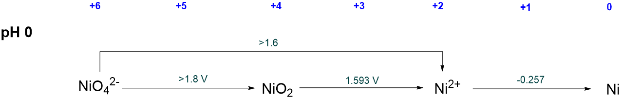
In such cases the relevant reduction potential should be calculated by taking into account the fact that since free energy is a state function, the free energy for formation of that oxidation state is the sum of the free energies of the steps described in the Latimer diagram. For example, to calculate \(NE^{\circ}\) for the formation of NiO₂, the following relationship may be used:

\[ \Delta G^{\circ}_{NiO_2 \rightarrow Ni} = \Delta G^{\circ}_{NiO_2 \rightarrow Ni^{2+}} + \Delta G^{\circ} _{Ni^{2+} \rightarrow Ni} \nonumber \]

But since \(\Delta G = -nF E^{\circ}\), where \(n\) is the number of electrons involved in each reduction, then the above expression may be rewritten as

\[ -n_{e^-,NiO_2 \rightarrow Ni}FE^{\circ}_{NiO_2 \rightarrow Ni} = -n_{e^-,NiO_2 \rightarrow Ni^{2+}}FE^{\circ}_{NiO_2 \rightarrow Ni^{2+}} + -n_{e^-,Ni^{2+} \rightarrow Ni}FE^{\circ} _{Ni^{2+} \rightarrow Ni} \nonumber \]

which may be further simplified by cancelling the Faraday constant, \(F\), from both sides, giving an expression for the desired value of \(NE^{\circ}\):

\[ -n_{e^-,NiO_2 \rightarrow Ni}E^{\circ}_{NiO_2 \rightarrow Ni} = NE^{\circ}_{Ni \rightarrow NiO_2} = -n_{e^-,NiO_2 \rightarrow Ni^{2+}}E^{\circ}_{NiO_2 \rightarrow Ni^{2+}} + -n_{e^-,Ni^{2+} \rightarrow Ni}E^{\circ} _{Ni^{2+} \rightarrow Ni} \nonumber \]

From this expression the value of \(NE^{\circ}_{Ni \rightarrow NiO_2}\) may be calculated by inserting the relevant reduction potentials and number of electrons:

\[ NE^{\circ}_{\sf{Ni \rightarrow NiO_2}} = 2 \times (+1.593 V) + 2 \times (-0.257 V) = +2.672 V \nonumber \]

For complex cases it can be helpful to tabulate the calculations, as is done in the following example.

Example \(\PageIndex{1}\): Calculating the Frost Diagram for nitrogen in aqueous acid

Calculate the acidic Frost diagram of nitrogen from the information given in the simplified acidic Latimer diagram for nitrogen given below.

Solution

The value of \(NE^{\circ}\) for each oxidation state is calculated as described in Table \(\PageIndex{1}\). The calculations follow the procedure:

1. Set \(NE^{\circ}\) = 0 for the free element.
2. Use \(NE^{\circ}\) = O.S. \(\times\) associated \(E^{\circ}\) to calculate \(NE^{\circ}\) for the lowest positive and negative oxidation states.
3. Iteratively use \( NE^{\circ}\) = \( NE^{\circ}_{\sf{last~~step}}\) + \(NE^{\circ}_{\sf{one~~lower~~oxidation~~state}}\) to calculate \(NE^{\circ}\) for all higher oxidation states.

Table \(\PageIndex{1}\): Calculation of \(NE^{\circ}\) for each oxidation state of nitrogen.

Oxidation State	Step	\(NE^{\circ}\) =	Calculated as the sum of the steps	Notes
5	N2 \(\rightarrow\) NO3^-	\(5 \times (E^{\circ}_{NO_3^- \rightarrow N_2})\)	\(\sf{N_2 \rightarrow N_2O_4 \rightarrow NO_3^-}\) \(NE^{\circ} = 1 \times E^{\circ}_{NO_3^- \rightarrow N_2O_4} +4 \times E^{\circ}_{N_2O_4 \rightarrow N_2}\) \(NE^{\circ} = 1 \times E^{\circ}_{NO_3^- \rightarrow N_2O_4} +NE^{\circ}_{+4~O.S.}\) \(NE^{\circ} = 1 \times 0.803 V + 5.426 V = 6.229 V\)	Calculate \(NE^{\circ}\) for the +4 oxidation state, NO, first. Then use it in this calculation.
4	N2 \(\rightarrow\) N2O4	\(4 \times (E^{\circ}_{N_2O_4 \rightarrow N_2})\)	\(\sf{N_2 \rightarrow HNO_2 \rightarrow N_2O_4}\) \(NE^{\circ} = 1 \times E^{\circ}_{HNO_2 \rightarrow NO} +3 \times E^{\circ}_{HNO_2 \rightarrow N_2}\) \(NE^{\circ} = 1 \times E^{\circ}_{N_2O_4 \rightarrow HNO_2} +NE^{\circ}_{+3~O.S.}\) \(NE^{\circ} = 1 \times 1.07 V + 4.356 V = 5.426 V\)	Calculate \(NE^{\circ}\) for the +3 oxidation state, NO, first. Then use it in this calculation.
3	N2 \(\rightarrow\) HNO2	\(3 \times (E^{\circ}_{HNO_2 \rightarrow N_2})\)	\(\sf{N_2 \rightarrow NO \rightarrow HNO_2}\) \(NE^{\circ} = 1 \times E^{\circ}_{HNO_2 \rightarrow NO} +2 \times E^{\circ}_{NO \rightarrow N_2}\) \(NE^{\circ} = 1 \times E^{\circ}_{NO \rightarrow N_2O} +NE^{\circ}_{+2~O.S.}\) \(NE^{\circ} = 1 \times 0.996 V + 3.36 V = 4.356 V\)	Calculate \(NE^{\circ}\) for the +2 oxidation state, NO, first. Then use it in this calculation.
2	N2 \(\rightarrow\) NO	\(2 \times (E^{\circ}_{NO \rightarrow N_2})\)	\(\sf{N_2 \rightarrow N_2O \rightarrow NO}\) \(NE^{\circ} = 1 \times E^{\circ}_{NO \rightarrow N_2O} +1 \times E^{\circ}_{N_2O \rightarrow N_2}\) \(NE^{\circ} = 1 \times E^{\circ}_{NO \rightarrow N_2O} +NE^{\circ}_{+1~O.S.}\) \(NE^{\circ} = 1 \times 1.59 V + 1.77 V = 3.36 V\)	Calculate \(NE^{\circ}\) for the +1 oxidation state, NO, first. Then use it in this calculation.
1	N2 \(\rightarrow\) N2O	\(1 \times E^{\circ}_{N_2O \rightarrow N_2}\)	\(\sf{N_2 \rightarrow N_2O}\) \(NE^{\circ} = 1 \times E^{\circ}_{N_2O \rightarrow N_2}\) \(NE^{\circ} = 1 \times +1.77 V = +1.77 V\)
0	None	0 V	\(NE^{\circ} = 0 V\) by definition.	Defined as 0 V
-1	N2 \(\rightarrow\) NH3OH^+	\((-1) \times E^{\circ}_{N_2 \rightarrow NH_3OH^+}\)	\(\sf{N_2 \rightarrow NH_3OH^+}\) \(NE^{\circ} = (-1) E^{\circ}_{N_2 \rightarrow NH_3OH^+}\) \(NE^{\circ} = (-1) \times (-1.87 V)= +1.87 V\)
-2	N2 \(\rightarrow\) N2H5^+	\((-2) \times E^{\circ}_{N_2 \rightarrow N_2H_5^+}\)	\(\sf{N_2 \rightarrow NH_3OH^+ \rightarrow N_2H_5^+}\) \(NE^{\circ} = (-1) \times E^{\circ}_{N_2\rightarrow NH_3OH^+} + (-1) E^{\circ}_{NH_3OH^+\rightarrow N_2H_5^+}\) \(NE^{\circ} = NE^{\circ}_{-1~O.S.} + (-1) E^{\circ}_{NH_3OH^+\rightarrow N_2H_5^+} \) \(NE^{\circ} = +1.87 V + (-1) \times 1.41 V = 0.46 V\)	Calculate \(NE^{\circ}\) for the -1 oxidation state, NO, first. Then use it in this calculation.
-3	N2 \(\rightarrow\) NH4^+	\((-3) \times E^{\circ}_{N_2 \rightarrow NH_4^+}\)	\(\sf{N_2 \rightarrow N_2H_5^+ \rightarrow NH_4^+}\) \(NE^{\circ} = (-1) E^{\circ}_{N_2\rightarrow N_2H_5^+} + (-1) E^{\circ}_{N_2H_5^+ \rightarrow NH_4^+}\) \(NE^{\circ} = NE^{\circ}_{-2~O.S.} + (-1) E^{\circ}_{N_2H_5^+ \rightarrow NH_4^+} \) \(NE^{\circ} = +0.46 V + (-1) \times 1.275 V = -0.815 V\)	Calculate \(NE^{\circ}\) for the -2 oxidation state, NO, first. Then use it in this calculation.

The resulting Frost diagram for acidic aqueous nitrogen is given below.

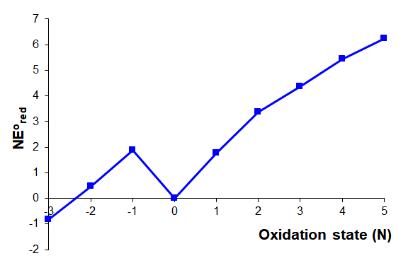
The figure above by Stephen Contakes is licensed under a Creative Commons Attribution 4.0 International License.

References

1. Unless otherwise noted all potentials are for strongly acidic solutions and taken from Bard, A. J.; Parsons, R.; Jordan, J. Standard potentials in aqueous solution. M. Dekker: New York, 1985.
2. This diagram is inspired by the similar diagram given in M. Gerken Chemistry 2810 Lecture Notes. Posted on classes.uleth.ca/200501/chem2...lecture_20.pdf
3. The estimated \( \sf{Fe^{6/3+}} \) reduction potential of +2.07 V used to construct the Frost diagram for the first row transition metals is taken from Huheey, J. E.; Keiter, E. A.; Keiter, R. L., Inorganic chemistry : principles of structure and reactivity. 4th ed.; HarperCollins College Publishers: New York, NY, 1993; pg. 596.
4. Lu, J.-B.; Jian, J.; Huang, W.; Lin, H.; Li, J.; Zhou, M., Experimental and theoretical identification of the Fe(vii) oxidation state in FeO4−. Physical Chemistry Chemical Physics 2016, 18 (45), 31125-31131.
5. In some pedagogical applications only the adjoining states are considered.

Contributors and Attributions

• Stephen Contakes, Westmont College