
17.2: Buffered Solutions
- Page ID
- 25184
\( \newcommand{\vecs}[1]{\overset { \scriptstyle \rightharpoonup} {\mathbf{#1}} } \)
\( \newcommand{\vecd}[1]{\overset{-\!-\!\rightharpoonup}{\vphantom{a}\smash {#1}}} \)
\( \newcommand{\id}{\mathrm{id}}\) \( \newcommand{\Span}{\mathrm{span}}\)
( \newcommand{\kernel}{\mathrm{null}\,}\) \( \newcommand{\range}{\mathrm{range}\,}\)
\( \newcommand{\RealPart}{\mathrm{Re}}\) \( \newcommand{\ImaginaryPart}{\mathrm{Im}}\)
\( \newcommand{\Argument}{\mathrm{Arg}}\) \( \newcommand{\norm}[1]{\| #1 \|}\)
\( \newcommand{\inner}[2]{\langle #1, #2 \rangle}\)
\( \newcommand{\Span}{\mathrm{span}}\)
\( \newcommand{\id}{\mathrm{id}}\)
\( \newcommand{\Span}{\mathrm{span}}\)
\( \newcommand{\kernel}{\mathrm{null}\,}\)
\( \newcommand{\range}{\mathrm{range}\,}\)
\( \newcommand{\RealPart}{\mathrm{Re}}\)
\( \newcommand{\ImaginaryPart}{\mathrm{Im}}\)
\( \newcommand{\Argument}{\mathrm{Arg}}\)
\( \newcommand{\norm}[1]{\| #1 \|}\)
\( \newcommand{\inner}[2]{\langle #1, #2 \rangle}\)
\( \newcommand{\Span}{\mathrm{span}}\) \( \newcommand{\AA}{\unicode[.8,0]{x212B}}\)
\( \newcommand{\vectorA}[1]{\vec{#1}} % arrow\)
\( \newcommand{\vectorAt}[1]{\vec{\text{#1}}} % arrow\)
\( \newcommand{\vectorB}[1]{\overset { \scriptstyle \rightharpoonup} {\mathbf{#1}} } \)
\( \newcommand{\vectorC}[1]{\textbf{#1}} \)
\( \newcommand{\vectorD}[1]{\overrightarrow{#1}} \)
\( \newcommand{\vectorDt}[1]{\overrightarrow{\text{#1}}} \)
\( \newcommand{\vectE}[1]{\overset{-\!-\!\rightharpoonup}{\vphantom{a}\smash{\mathbf {#1}}}} \)
\( \newcommand{\vecs}[1]{\overset { \scriptstyle \rightharpoonup} {\mathbf{#1}} } \)
\( \newcommand{\vecd}[1]{\overset{-\!-\!\rightharpoonup}{\vphantom{a}\smash {#1}}} \)
\(\newcommand{\avec}{\mathbf a}\) \(\newcommand{\bvec}{\mathbf b}\) \(\newcommand{\cvec}{\mathbf c}\) \(\newcommand{\dvec}{\mathbf d}\) \(\newcommand{\dtil}{\widetilde{\mathbf d}}\) \(\newcommand{\evec}{\mathbf e}\) \(\newcommand{\fvec}{\mathbf f}\) \(\newcommand{\nvec}{\mathbf n}\) \(\newcommand{\pvec}{\mathbf p}\) \(\newcommand{\qvec}{\mathbf q}\) \(\newcommand{\svec}{\mathbf s}\) \(\newcommand{\tvec}{\mathbf t}\) \(\newcommand{\uvec}{\mathbf u}\) \(\newcommand{\vvec}{\mathbf v}\) \(\newcommand{\wvec}{\mathbf w}\) \(\newcommand{\xvec}{\mathbf x}\) \(\newcommand{\yvec}{\mathbf y}\) \(\newcommand{\zvec}{\mathbf z}\) \(\newcommand{\rvec}{\mathbf r}\) \(\newcommand{\mvec}{\mathbf m}\) \(\newcommand{\zerovec}{\mathbf 0}\) \(\newcommand{\onevec}{\mathbf 1}\) \(\newcommand{\real}{\mathbb R}\) \(\newcommand{\twovec}[2]{\left[\begin{array}{r}#1 \\ #2 \end{array}\right]}\) \(\newcommand{\ctwovec}[2]{\left[\begin{array}{c}#1 \\ #2 \end{array}\right]}\) \(\newcommand{\threevec}[3]{\left[\begin{array}{r}#1 \\ #2 \\ #3 \end{array}\right]}\) \(\newcommand{\cthreevec}[3]{\left[\begin{array}{c}#1 \\ #2 \\ #3 \end{array}\right]}\) \(\newcommand{\fourvec}[4]{\left[\begin{array}{r}#1 \\ #2 \\ #3 \\ #4 \end{array}\right]}\) \(\newcommand{\cfourvec}[4]{\left[\begin{array}{c}#1 \\ #2 \\ #3 \\ #4 \end{array}\right]}\) \(\newcommand{\fivevec}[5]{\left[\begin{array}{r}#1 \\ #2 \\ #3 \\ #4 \\ #5 \\ \end{array}\right]}\) \(\newcommand{\cfivevec}[5]{\left[\begin{array}{c}#1 \\ #2 \\ #3 \\ #4 \\ #5 \\ \end{array}\right]}\) \(\newcommand{\mattwo}[4]{\left[\begin{array}{rr}#1 \amp #2 \\ #3 \amp #4 \\ \end{array}\right]}\) \(\newcommand{\laspan}[1]{\text{Span}\{#1\}}\) \(\newcommand{\bcal}{\cal B}\) \(\newcommand{\ccal}{\cal C}\) \(\newcommand{\scal}{\cal S}\) \(\newcommand{\wcal}{\cal W}\) \(\newcommand{\ecal}{\cal E}\) \(\newcommand{\coords}[2]{\left\{#1\right\}_{#2}}\) \(\newcommand{\gray}[1]{\color{gray}{#1}}\) \(\newcommand{\lgray}[1]{\color{lightgray}{#1}}\) \(\newcommand{\rank}{\operatorname{rank}}\) \(\newcommand{\row}{\text{Row}}\) \(\newcommand{\col}{\text{Col}}\) \(\renewcommand{\row}{\text{Row}}\) \(\newcommand{\nul}{\text{Nul}}\) \(\newcommand{\var}{\text{Var}}\) \(\newcommand{\corr}{\text{corr}}\) \(\newcommand{\len}[1]{\left|#1\right|}\) \(\newcommand{\bbar}{\overline{\bvec}}\) \(\newcommand{\bhat}{\widehat{\bvec}}\) \(\newcommand{\bperp}{\bvec^\perp}\) \(\newcommand{\xhat}{\widehat{\xvec}}\) \(\newcommand{\vhat}{\widehat{\vvec}}\) \(\newcommand{\uhat}{\widehat{\uvec}}\) \(\newcommand{\what}{\widehat{\wvec}}\) \(\newcommand{\Sighat}{\widehat{\Sigma}}\) \(\newcommand{\lt}{<}\) \(\newcommand{\gt}{>}\) \(\newcommand{\amp}{&}\) \(\definecolor{fillinmathshade}{gray}{0.9}\)- To understand how adding a common ion affects the position of an acid–base equilibrium.
- To know how to use the Henderson-Hasselbalch approximation to calculate the pH of a buffer.
Buffers are solutions that maintain a relatively constant pH when an acid or a base is added. They therefore protect, or “buffer,” other molecules in solution from the effects of the added acid or base. Buffers contain either a weak acid (\(HA\)) and its conjugate base \((A^−\)) or a weak base (\(B\)) and its conjugate acid (\(BH^+\)), and they are critically important for the proper functioning of biological systems. In fact, every biological fluid is buffered to maintain its physiological pH.
The Common Ion Effect: Weak Acids Combined with Conjugate Bases
To understand how buffers work, let’s look first at how the ionization equilibrium of a weak acid is affected by adding either the conjugate base of the acid or a strong acid (a source of \(\ce{H^{+}}\)). Le Chatelier’s principle can be used to predict the effect on the equilibrium position of the solution. A typical buffer used in biochemistry laboratories contains acetic acid and a salt such as sodium acetate. The dissociation reaction of acetic acid is as follows:
\[\ce{CH3COOH (aq) <=> CH3COO^{−} (aq) + H^{+} (aq)} \label{Eq1} \]
and the equilibrium constant expression is as follows:
\[K_a=\dfrac{[\ce{H^{+}}][\ce{CH3COO^{-}}]}{[\ce{CH3CO2H}]} \label{Eq2} \]
Sodium acetate (\(\ce{CH_3CO_2Na}\)) is a strong electrolyte that ionizes completely in aqueous solution to produce \(\ce{Na^{+}}\) and \(\ce{CH3CO2^{−}}\) ions. If sodium acetate is added to a solution of acetic acid, Le Chatelier’s principle predicts that the equilibrium in Equation \ref{Eq1} will shift to the left, consuming some of the added \(\ce{CH_3COO^{−}}\) and some of the \(\ce{H^{+}}\) ions originally present in solution.
Because \(\ce{Na^{+}}\) is a spectator ion, it has no effect on the position of the equilibrium and can be ignored. The addition of sodium acetate produces a new equilibrium composition, in which \([\ce{H^{+}}]\) is less than the initial value. Because \([\ce{H^{+}}]\) has decreased, the pH will be higher. Thus adding a salt of the conjugate base to a solution of a weak acid increases the pH. This makes sense because sodium acetate is a base, and adding any base to a solution of a weak acid should increase the pH.
If we instead add a strong acid such as \(\ce{HCl}\) to the system, \([\ce{H^{+}}]\) increases. Once again the equilibrium is temporarily disturbed, but the excess \(\ce{H^{+}}\) ions react with the conjugate base (\(\ce{CH_3CO_2^{−}}\)), whether from the parent acid or sodium acetate, to drive the equilibrium to the left. The net result is a new equilibrium composition that has a lower [\(\ce{CH_3CO_2^{−}}\)] than before. In both cases, only the equilibrium composition has changed; the ionization constant \(K_a\) for acetic acid remains the same. Adding a strong electrolyte that contains one ion in common with a reaction system that is at equilibrium, in this case \(\ce{CH3CO2^{−}}\), will therefore shift the equilibrium in the direction that reduces the concentration of the common ion. The shift in equilibrium is via the common ion effect.
Adding a common ion to a system at equilibrium affects the equilibrium composition, but not the ionization constant.
A 0.150 M solution of formic acid at 25°C (pKa = 3.75) has a pH of 2.28 and is 3.5% ionized.
- Is there a change to the pH of the solution if enough solid sodium formate is added to make the final formate concentration 0.100 M (assume that the formic acid concentration does not change)?
- What percentage of the formic acid is ionized if 0.200 M HCl is added to the system?
Given: solution concentration and pH, \(pK_a\), and percent ionization of acid; final concentration of conjugate base or strong acid added
Asked for: pH and percent ionization of formic acid
Strategy:
- Write a balanced equilibrium equation for the ionization equilibrium of formic acid. Tabulate the initial concentrations, the changes, and the final concentrations.
- Substitute the expressions for the final concentrations into the expression for Ka. Calculate \([\ce{H^{+}}]\) and the pH of the solution.
- Construct a table of concentrations for the dissociation of formic acid. To determine the percent ionization, determine the anion concentration, divide it by the initial concentration of formic acid, and multiply the result by 100.
Solution:
A Because sodium formate is a strong electrolyte, it ionizes completely in solution to give formate and sodium ions. The \(\ce{Na^{+}}\) ions are spectator ions, so they can be ignored in the equilibrium equation. Because water is both a much weaker acid than formic acid and a much weaker base than formate, the acid–base properties of the solution are determined solely by the formic acid ionization equilibrium:
\[\ce{HCO2H (aq) <=> HCO^{−}2 (aq) + H^{+} (aq)} \nonumber \]
The initial concentrations, the changes in concentration that occur as equilibrium is reached, and the final concentrations can be tabulated.
| ICE | \([HCO_2H (aq) ]\) | \([H^+ (aq) ]\) | \([HCO^−_2 (aq) ]\) |
|---|---|---|---|
| Initial | 0.150 | \(1.00 \times 10^{−7}\) | 0.100 |
| Change | −x | +x | +x |
| Equilibrium | (0.150 − x) | x | (0.100 + x) |
B We substitute the expressions for the final concentrations into the equilibrium constant expression and make our usual simplifying assumptions, so
\[\begin{align*} K_a=\dfrac{[H^+][HCO_2^−]}{[HCO_2H]} &=\dfrac{(x)(0.100+x)}{0.150−x} \\[4pt] &\approx \dfrac{x(0.100)}{0.150} \\[4pt] &\approx 10^{−3.75} \\[4pt] &\approx 1.8 \times 10^{−4} \end{align*} \nonumber \]
Rearranging and solving for \(x\),
\[\begin{align*} x &=(1.8 \times 10^{−4}) \times \dfrac{0.150 \;M}{ 0.100 \;M} \\[4pt] &=2.7 \times 10^{−4}\\[4pt] &=[H^+] \end{align*} \nonumber \]
The value of \(x\) is small compared with 0.150 or 0.100 M, so our assumption about the extent of ionization is justified. Moreover,
\[K_aC_{HA} = (1.8 \times 10^{−4})(0.150) = 2.7 \times 10^{−5} \nonumber \]
which is greater than \(1.0 \times 10^{−6}\), so again, our assumption is justified. The final pH is:
\[pH= −\log(2.7 \times 10^{−4}) = 3.57 \nonumber \]
compared with the initial value of 2.29. Thus adding a salt containing the conjugate base of the acid has increased the pH of the solution, as we expect based on Le Chatelier’s principle; the stress on the system has been relieved by the consumption of \(\ce{H^{+}}\) ions, driving the equilibrium to the left.
C Because \(HCl\) is a strong acid, it ionizes completely, and chloride is a spectator ion that can be neglected. Thus the only relevant acid–base equilibrium is again the dissociation of formic acid, and initially the concentration of formate is zero. We can construct a table of initial concentrations, changes in concentration, and final concentrations.
\[HCO_2H (aq) \leftrightharpoons H^+ (aq) +HCO^−_2 (aq) \nonumber \]
| \([HCO_2H (aq) ]\) | \([H^+ (aq) ]\) | \([HCO^−_2 (aq) ]\) | |
|---|---|---|---|
| initial | 0.150 | 0.200 | 0 |
| change | −x | +x | +x |
| final | (0.150 − x) | (0.200 + x) | x |
To calculate the percentage of formic acid that is ionized under these conditions, we have to determine the final \([\ce{HCO2^{-}}]\). We substitute final concentrations into the equilibrium constant expression and make the usual simplifying assumptions, so
\[K_a=\dfrac{[H^+][HCO_2^−]}{[HCO_2H]}=\dfrac{(0.200+x)(x)}{0.150−x} \approx \dfrac{x(0.200)}{0.150}=1.80 \times 10^{−4} \nonumber \]
Rearranging and solving for \(x\),
\[\begin{align*} x &=(1.80 \times 10^{−4}) \times \dfrac{ 0.150\; M}{ 0.200\; M} \\[4pt] &=1.35 \times 10^{−4}=[HCO_2^−] \end{align*} \nonumber \]
Once again, our simplifying assumptions are justified. The percent ionization of formic acid is as follows:
\[\text{percent ionization}=\dfrac{1.35 \times 10^{−4} \;M} {0.150\; M} \times 100\%=0.0900\% \nonumber \]
Adding the strong acid to the solution, as shown in the table, decreased the percent ionization of formic acid by a factor of approximately 38 (3.45%/0.0900%). Again, this is consistent with Le Chatelier’s principle: adding \(\ce{H^{+}}\) ions drives the dissociation equilibrium to the left.
A 0.225 M solution of ethylamine (\(\ce{CH3CH2NH2}\) with \(pK_b = 3.19\)) has a pH of 12.08 and a percent ionization of 5.4% at 20°C. Calculate the following:
- the pH of the solution if enough solid ethylamine hydrochloride (\(\ce{EtNH3Cl}\)) is added to make the solution 0.100 M in \(\ce{EtNH3^{+}}\)
- the percentage of ethylamine that is ionized if enough solid \(\ce{NaOH}\) is added to the original solution to give a final concentration of 0.050 M \(\ce{NaOH}\)
- Answer a
-
11.16
- Answer b
-
1.3%
A Video Discussing the Common Ion Effect: The Common Ion Effecr(opens in new window) [youtu.be]
The Common Ion Effect: Weak Bases Combined with Conjugate Acids
Now let’s suppose we have a buffer solution that contains equimolar concentrations of a weak base (\(B\)) and its conjugate acid (\(BH^+\)). The general equation for the ionization of a weak base is as follows:
\[B (aq) +H_2O (l) \leftrightharpoons BH^+ (aq) +OH^− (aq) \label{Eq3} \]
If the equilibrium constant for the reaction as written in Equation \(\ref{Eq3}\) is small, for example \(K_b = 10^{−5}\), then the equilibrium constant for the reverse reaction is very large: \(K = \dfrac{1}{K_b} = 10^5\). Adding a strong base such as \(OH^-\) to the solution therefore causes the equilibrium in Equation \(\ref{Eq3}\) to shift to the left, consuming the added \(OH^-\). As a result, the \(OH^-\) ion concentration in solution remains relatively constant, and the pH of the solution changes very little. Le Chatelier’s principle predicts the same outcome: when the system is stressed by an increase in the \(OH^-\) ion concentration, the reaction will proceed to the left to counteract the stress.
If the \(pK_b\) of the base is 5.0, the \(pK_a\) of its conjugate acid is
\[pK_a = pK_w − pK_b = 14.0 – 5.0 = 9.0. \nonumber \]
Thus the equilibrium constant for ionization of the conjugate acid is even smaller than that for ionization of the base. The ionization reaction for the conjugate acid of a weak base is written as follows:
\[BH^+ (aq) +H_2O (l) \leftrightharpoons B (aq) +H_3O^+ (aq) \label{Eq4} \]
Again, the equilibrium constant for the reverse of this reaction is very large: K = 1/Ka = 109. If a strong acid is added, it is neutralized by reaction with the base as the reaction in Equation \(\ref{Eq4}\) shifts to the left. As a result, the \(H^+\) ion concentration does not increase very much, and the pH changes only slightly. In effect, a buffer solution behaves somewhat like a sponge that can absorb \(H^+\) and \(OH^-\) ions, thereby preventing large changes in pH when appreciable amounts of strong acid or base are added to a solution.
Buffers are characterized by the pH range over which they can maintain a more or less constant pH and by their buffer capacity, the amount of strong acid or base that can be absorbed before the pH changes significantly. Although the useful pH range of a buffer depends strongly on the chemical properties of the weak acid and weak base used to prepare the buffer (i.e., on \(K\)), its buffer capacity depends solely on the concentrations of the species in the buffered solution. The more concentrated the buffer solution, the greater its buffer capacity. As illustrated in Figure \(\PageIndex{1}\), when \(NaOH\) is added to solutions that contain different concentrations of an acetic acid/sodium acetate buffer, the observed change in the pH of the buffer is inversely proportional to the concentration of the buffer. If the buffer capacity is 10 times larger, then the buffer solution can absorb 10 times more strong acid or base before undergoing a significant change in pH.
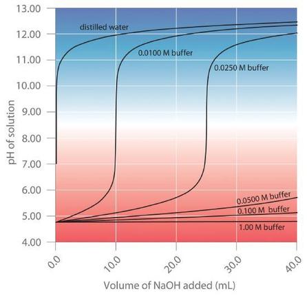
A buffer maintains a relatively constant pH when acid or base is added to a solution. The addition of even tiny volumes of 0.10 M \(NaOH\) to 100.0 mL of distilled water results in a very large change in pH. As the concentration of a 50:50 mixture of sodium acetate/acetic acid buffer in the solution is increased from 0.010 M to 1.00 M, the change in the pH produced by the addition of the same volume of \(NaOH\) solution decreases steadily. For buffer concentrations of at least 0.500 M, the addition of even 25 mL of the \(NaOH\) solution results in only a relatively small change in pH.
Calculating the pH of a Buffer
The pH of a buffer can be calculated from the concentrations of the weak acid and the weak base used to prepare it, the concentration of the conjugate base and conjugate acid, and the \(pK_a\) or \(pK_b\) of the weak acid or weak base. The procedure is analogous to that used in Example \(\PageIndex{1}\) to calculate the pH of a solution containing known concentrations of formic acid and formate.
An alternative method frequently used to calculate the pH of a buffer solution is based on a rearrangement of the equilibrium equation for the dissociation of a weak acid. The simplified ionization reaction is \(HA \leftrightharpoons H^+ + A^−\), for which the equilibrium constant expression is as follows:
\[K_a=\dfrac{[H^+][A^-]}{[HA]} \label{Eq5} \]
This equation can be rearranged as follows:
\[[H^+]=K_a\dfrac{[HA]}{[A^−]} \label{Eq6} \]
Taking the logarithm of both sides and multiplying both sides by −1,
\[ \begin{align} −\log[H^+] &=−\log K_a−\log\left(\dfrac{[HA]}{[A^−]}\right) \\[4pt] &=−\log{K_a}+\log\left(\dfrac{[A^−]}{[HA]}\right) \label{Eq7} \end{align} \]
Replacing the negative logarithms in Equation \(\ref{Eq7}\),
\[pH=pK_a+\log \left( \dfrac{[A^−]}{[HA]} \right) \label{Eq8} \]
or, more generally,
\[pH=pK_a+\log\left(\dfrac{[base]}{[acid]}\right) \label{Eq9} \]
Equation \(\ref{Eq8}\) and Equation \(\ref{Eq9}\) are both forms of the Henderson-Hasselbalch approximation, named after the two early 20th-century chemists who first noticed that this rearranged version of the equilibrium constant expression provides an easy way to calculate the pH of a buffer solution. In general, the validity of the Henderson-Hasselbalch approximation may be limited to solutions whose concentrations are at least 100 times greater than their \(K_a\) values.
There are three special cases where the Henderson-Hasselbalch approximation is easily interpreted without the need for calculations:
- \([base] = [acid]\): Under these conditions, \[\dfrac{[base]}{[acid]} = 1 \nonumber \] in Equation \ref{Eq9}. Because \(\log 1 = 0\), \[pH = pK_a \nonumber \] regardless of the actual concentrations of the acid and base. Recall that this corresponds to the midpoint in the titration of a weak acid or a weak base.
- \([base]/[acid] = 10\): In Equation \(\ref{Eq9}\), because \(\log 10 = 1\), \[pH = pK_a + 1. \nonumber \]
- \([base]/[acid] = 100\): In Equation \(\ref{Eq9}\), because \(\log 100 = 2\), \[pH = pK_a + 2. \nonumber \]
Each time we increase the [base]/[acid] ratio by 10, the pH of the solution increases by 1 pH unit. Conversely, if the [base]/[acid] ratio is 0.1, then pH = \(pK_a\) − 1. Each additional factor-of-10 decrease in the [base]/[acid] ratio causes the pH to decrease by 1 pH unit.
If [base] = [acid] for a buffer, then pH = \(pK_a\). Changing this ratio by a factor of 10 either way changes the pH by ±1 unit.
What is the pH of a solution that contains
- 0.135 M \(\ce{HCO2H}\) and 0.215 M \(\ce{HCO2Na}\)? (The \(pK_a\) of formic acid is 3.75.)
- 0.0135 M \(\ce{HCO2H}\) and 0.0215 M \(\ce{HCO2Na}\)?
- 0.119 M pyridine and 0.234 M pyridine hydrochloride? (The \(pK_b\) of pyridine is 8.77.)
Given: concentration of acid, conjugate base, and \(pK_a\); concentration of base, conjugate acid, and \(pK_b\)
Asked for: pH
Strategy:
Substitute values into either form of the Henderson-Hasselbalch approximation (Equations \ref{Eq8} or \ref{Eq9}) to calculate the pH.
Solution:
According to the Henderson-Hasselbalch approximation (Equation \ref{Eq8}), the pH of a solution that contains both a weak acid and its conjugate base is
\[pH = pK_a + \log([A−]/[HA]). \nonumber \]
A
Inserting the given values into the equation,
\[\begin{align*} pH &=3.75+\log\left(\dfrac{0.215}{0.135}\right) \\[4pt] &=3.75+\log 1.593 \\[4pt] &=3.95 \end{align*} \nonumber \]
This result makes sense because the \([A^−]/[HA]\) ratio is between 1 and 10, so the pH of the buffer must be between the \(pK_a\) (3.75) and \(pK_a + 1\), or 4.75.
B
This is identical to part (a), except for the concentrations of the acid and the conjugate base, which are 10 times lower. Inserting the concentrations into the Henderson-Hasselbalch approximation,
\[\begin{align*} pH &=3.75+\log\left(\dfrac{0.0215}{0.0135}\right) \\[4pt] &=3.75+\log 1.593 \\[4pt] &=3.95 \end{align*} \nonumber \]
This result is identical to the result in part (a), which emphasizes the point that the pH of a buffer depends only on the ratio of the concentrations of the conjugate base and the acid, not on the magnitude of the concentrations. Because the [A−]/[HA] ratio is the same as in part (a), the pH of the buffer must also be the same (3.95).
C
In this case, we have a weak base, pyridine (Py), and its conjugate acid, the pyridinium ion (\(HPy^+\)). We will therefore use Equation \(\ref{Eq9}\), the more general form of the Henderson-Hasselbalch approximation, in which “base” and “acid” refer to the appropriate species of the conjugate acid–base pair. We are given [base] = [Py] = 0.119 M and \([acid] = [HPy^{+}] = 0.234\, M\). We also are given \(pK_b = 8.77\) for pyridine, but we need \(pK_a\) for the pyridinium ion. Recall from Equation 16.23 that the \(pK_b\) of a weak base and the \(pK_a\) of its conjugate acid are related:
\[pK_a + pK_b = pK_w. \nonumber \]
Thus \(pK_a\) for the pyridinium ion is \(pK_w − pK_b = 14.00 − 8.77 = 5.23\). Substituting this \(pK_a\) value into the Henderson-Hasselbalch approximation,
\[\begin{align*} pH=pK_a+\log \left(\dfrac{[base]}{[acid]}\right) \\[4pt] &=5.23+\log\left(\dfrac{0.119}{0.234}\right) \\[4pt] & =5.23 −0.294 \\[4pt] &=4.94 \end{align*} \nonumber \]
Once again, this result makes sense: the \([B]/[BH^+]\) ratio is about 1/2, which is between 1 and 0.1, so the final pH must be between the \(pK_a\) (5.23) and \(pK_a − 1\), or 4.23.
What is the pH of a solution that contains
- 0.333 M benzoic acid and 0.252 M sodium benzoate?
- 0.050 M trimethylamine and 0.066 M trimethylamine hydrochloride?
The \(pK_a\) of benzoic acid is 4.20, and the \(pK_b\) of trimethylamine is also 4.20.
- Answer a
-
4.08
- Answer b
-
9.68
A Video Discussing Using the Henderson Hasselbalch Equation: Using the Henderson Hasselbalch Equation(opens in new window) [youtu.be] (opens in new window)
The Henderson-Hasselbalch approximation ((Equation \(\ref{Eq8}\)) can also be used to calculate the pH of a buffer solution after adding a given amount of strong acid or strong base, as demonstrated in Example \(\PageIndex{3}\).
The buffer solution in Example \(\PageIndex{2}\) contained 0.135 M \(\ce{HCO2H}\) and 0.215 M \(\ce{HCO2Na}\) and had a pH of 3.95.
- What is the final pH if 5.00 mL of 1.00 M \(HCl\) are added to 100 mL of this solution?
- What is the final pH if 5.00 mL of 1.00 M \(NaOH\) are added?
Given: composition and pH of buffer; concentration and volume of added acid or base
Asked for: final pH
Strategy:
- Calculate the amounts of formic acid and formate present in the buffer solution using the procedure from Example \(\PageIndex{1}\). Then calculate the amount of acid or base added.
- Construct a table showing the amounts of all species after the neutralization reaction. Use the final volume of the solution to calculate the concentrations of all species. Finally, substitute the appropriate values into the Henderson-Hasselbalch approximation (Equation \ref{Eq9}) to obtain the pH.
Solution:
The added \(\ce{HCl}\) (a strong acid) or \(\ce{NaOH}\) (a strong base) will react completely with formate (a weak base) or formic acid (a weak acid), respectively, to give formic acid or formate and water. We must therefore calculate the amounts of formic acid and formate present after the neutralization reaction.
A We begin by calculating the millimoles of formic acid and formate present in 100 mL of the initial pH 3.95 buffer:
\[ 100 \, \cancel{mL} \left( \dfrac{0.135 \, mmol\; \ce{HCO2H}}{\cancel{mL}} \right) = 13.5\, mmol\, \ce{HCO2H} \nonumber \]
\[ 100\, \cancel{mL } \left( \dfrac{0.215 \, mmol\; \ce{HCO2^{-}}}{\cancel{mL}} \right) = 21.5\, mmol\, \ce{HCO2^{-}} \nonumber \]
The millimoles of \(\ce{H^{+}}\) in 5.00 mL of 1.00 M \(\ce{HCl}\) is as follows:
\[ 5.00 \, \cancel{mL } \left( \dfrac{1.00 \,mmol\; \ce{H^{+}}}{\cancel{mL}} \right) = 5\, mmol\, \ce{H^{+}} \nonumber \]
B Next, we construct a table of initial amounts, changes in amounts, and final amounts:
\[\ce{HCO^{2−}(aq) + H^{+} (aq) <=> HCO2H (aq)} \nonumber \]
| \(HCO^{2−} (aq) \) | \(H^+ (aq) \) | \(HCO_2H (aq) \) | |
|---|---|---|---|
| Initial | 21.5 mmol | 5.00 mmol | 13.5 mmol |
| Change | −5.00 mmol | −5.00 mmol | +5.00 mmol |
| Final | 16.5 mmol | ∼0 mmol | 18.5 mmol |
The final amount of \(H^+\) in solution is given as “∼0 mmol.” For the purposes of the stoichiometry calculation, this is essentially true, but remember that the point of the problem is to calculate the final \([H^+]\) and thus the pH. We now have all the information we need to calculate the pH. We can use either the lengthy procedure of Example \(\PageIndex{1}\) or the Henderson–Hasselbach approximation. Because we have performed many equilibrium calculations in this chapter, we’ll take the latter approach. The Henderson-Hasselbalch approximation requires the concentrations of \(HCO_2^−\) and \(HCO_2H\), which can be calculated using the number of millimoles (\(n\)) of each and the total volume (\(VT\)). Substituting these values into the Henderson-Hasselbalch approximation (Equation \(\ref{Eq9}\)):
\[\begin{align*} pH &=pK_a+\log \left( \dfrac{[HCO_2^−]}{[HCO_2H]} \right) \\[4pt] &=pK_a+\log\left(\dfrac{n_{HCO_2^−}/V_f}{n_{HCO_2H}/V_f}\right) \\[4pt] &=pK_a+\log \left(\dfrac{n_{HCO_2^−}}{n_{HCO_2H}}\right) \end{align*} \nonumber \]
Because the total volume appears in both the numerator and denominator, it cancels. We therefore need to use only the ratio of the number of millimoles of the conjugate base to the number of millimoles of the weak acid. So
\[\begin{align*} pH &=pK_a+\log\left(\dfrac{n_{HCO_2^−}}{n_{HCO_2H}}\right) \\[4pt] &=3.75+\log\left(\dfrac{16.5\; mmol}{18.5\; mmol}\right) \\[4pt] &=3.75 −0.050=3.70 \end{align*} \nonumber \]
Once again, this result makes sense on two levels. First, the addition of \(HCl \)has decreased the pH from 3.95, as expected. Second, the ratio of \(HCO_2^−\) to \(HCO_2H\) is slightly less than 1, so the pH should be between the \(pK_a\) and \(pK_a\) − 1.
A The procedure for solving this part of the problem is exactly the same as that used in part (a). We have already calculated the numbers of millimoles of formic acid and formate in 100 mL of the initial pH 3.95 buffer: 13.5 mmol of \(HCO_2H\) and 21.5 mmol of \(HCO_2^−\). The number of millimoles of \(OH^-\) in 5.00 mL of 1.00 M \(NaOH\) is as follows:
B With this information, we can construct a table of initial amounts, changes in amounts, and final amounts.
\[\ce{HCO2H (aq) + OH^{−} (aq) <=> HCO^{−}2 (aq) + H2O (l)} \nonumber \]
| \(HCO_2H (aq) \) | \(OH^−\) | \(HCO^−_2 (aq) \) | |
|---|---|---|---|
| Initial | 13.5 mmol | 5.00 mmol | 21.5 mmol |
| Change | −5.00 mmol | −5.00 mmol | +5.00 mmol |
| Final | 8.5 mmol | ∼0 mmol | 26.5 mmol |
The final amount of \(OH^-\) in solution is not actually zero; this is only approximately true based on the stoichiometric calculation. We can calculate the final pH by inserting the numbers of millimoles of both \(HCO_2^−\) and \(HCO_2H\) into the simplified Henderson-Hasselbalch expression used in part (a) because the volume cancels:
\[\begin{align*} pH &=pK_a+\log \left(\dfrac{n_{HCO_2^−}}{n_{HCO_2H}}\right) \\[4pt] &=3.75+\log \left(\dfrac{26.5\; mmol}{8.5\; mmol} \right) \\[4pt] &=3.75+0.494 =4.24 \end{align*} \nonumber \]
Once again, this result makes chemical sense: the pH has increased, as would be expected after adding a strong base, and the final pH is between the \(pK_a\) and \(pK_a\) + 1, as expected for a solution with a \(HCO_2^−/HCO_2H\) ratio between 1 and 10.
The buffer solution from Example \(\PageIndex{2}\) contained 0.119 M pyridine and 0.234 M pyridine hydrochloride and had a pH of 4.94.
- What is the final pH if 12.0 mL of 1.5 M \(\ce{NaOH}\) are added to 250 mL of this solution?
- What is the final pH if 12.0 mL of 1.5 M \(\ce{HCl}\) are added?
- Answer a
-
5.30
- Answer b
-
4.42
Only the amounts (in moles or millimoles) of the acidic and basic components of the buffer are needed to use the Henderson-Hasselbalch approximation, not their concentrations.
A Video Discussing the Change in pH with the Addition of a Strong Acid to a Buffer: The Change in pH with the Addition of a Strong Acid to a Buffer(opens in new window) [youtu.be]
The Change in pH with the Addition of a Strong Base to a Buffer:
The Change in pH with the Addition of a Strong Base to a Buffer (opens in new window) [youtu.be]
The results obtained in Example \(\PageIndex{3}\) and its corresponding exercise demonstrate how little the pH of a well-chosen buffer solution changes despite the addition of a significant quantity of strong acid or strong base. Suppose we had added the same amount of \(HCl\) or \(NaOH\) solution to 100 mL of an unbuffered solution at pH 3.95 (corresponding to \(1.1 \times 10^{−4}\) M HCl). In this case, adding 5.00 mL of 1.00 M \(HCl\) would lower the final pH to 1.32 instead of 3.70, whereas adding 5.00 mL of 1.00 M \(NaOH\) would raise the final pH to 12.68 rather than 4.24. (Try verifying these values by doing the calculations yourself.) Thus the presence of a buffer significantly increases the ability of a solution to maintain an almost constant pH.
The most effective buffers contain equal concentrations of an acid and its conjugate base.
A buffer that contains approximately equal amounts of a weak acid and its conjugate base in solution is equally effective at neutralizing either added base or added acid. This is shown in Figure \(\PageIndex{2}\) for an acetic acid/sodium acetate buffer. Adding a given amount of strong acid shifts the system along the horizontal axis to the left, whereas adding the same amount of strong base shifts the system the same distance to the right. In either case, the change in the ratio of \(CH_3CO_2^−\) to \(CH_3CO_2H\) from 1:1 reduces the buffer capacity of the solution.

Figure \(\PageIndex{2}\): Distribution Curve Showing the Fraction of Acetic Acid Molecules and Acetate Ions as a Function of pH in a Solution of Acetic Acid. The pH range over which the acetic acid/sodium acetate system is an effective buffer (the darker shaded region) corresponds to the region in which appreciable concentrations of both species are present (pH 3.76–5.76, corresponding to \(pH = pK_a \pm 1\)). (CC BY-SA-NC; Anonymous by request)
A Video Discussing The Buffer Region: The Buffer Region (opens in new window) [youtu.be]
The Relationship between Titrations and Buffers
There is a strong correlation between the effectiveness of a buffer solution and the titration curves discussed in Section 16.5. Consider the schematic titration curve of a weak acid with a strong base shown in Figure \(\PageIndex{3}\). As indicated by the labels, the region around \(pK_a\) corresponds to the midpoint of the titration, when approximately half the weak acid has been neutralized. This portion of the titration curve corresponds to a buffer: it exhibits the smallest change in pH per increment of added strong base, as shown by the nearly horizontal nature of the curve in this region. The nearly flat portion of the curve extends only from approximately a pH value of 1 unit less than the \(pK_a\) to approximately a pH value of 1 unit greater than the \(pK_a\), which is why buffer solutions usually have a pH that is within ±1 pH units of the \(pK_a\) of the acid component of the buffer.

This schematic plot of pH for the titration of a weak acid with a strong base shows the nearly flat region of the titration curve around the midpoint, which corresponds to the formation of a buffer. At the lower left, the pH of the solution is determined by the equilibrium for dissociation of the weak acid; at the upper right, the pH is determined by the equilibrium for reaction of the conjugate base with water.
In the region of the titration curve at the lower left, before the midpoint, the acid–base properties of the solution are dominated by the equilibrium for dissociation of the weak acid, corresponding to \(K_a\). In the region of the titration curve at the upper right, after the midpoint, the acid–base properties of the solution are dominated by the equilibrium for reaction of the conjugate base of the weak acid with water, corresponding to \(K_b\). However, we can calculate either \(K_a\) or \(K_b\) from the other because they are related by \(K_w\).
Metabolic processes produce large amounts of acids and bases, yet organisms are able to maintain an almost constant internal pH because their fluids contain buffers. This is not to say that the pH is uniform throughout all cells and tissues of a mammal. The internal pH of a red blood cell is about 7.2, but the pH of most other kinds of cells is lower, around 7.0. Even within a single cell, different compartments can have very different pH values. For example, one intracellular compartment in white blood cells has a pH of around 5.0.
Because no single buffer system can effectively maintain a constant pH value over the entire physiological range of approximately pH 5.0 to 7.4, biochemical systems use a set of buffers with overlapping ranges. The most important of these is the \(\ce{CO2}/\ce{HCO3^{−}}\) system, which dominates the buffering action of blood plasma.
The acid–base equilibrium in the \(\ce{CO2}/\ce{HCO3^{−}}\) buffer system is usually written as follows:
\[\ce{H2CO3 (aq) <=> H^{+} (aq) + HCO^{-}3 (aq)} \label{Eq10} \]
with \(K_a = 4.5 \times 10^{−7}\) and \(pK_a = 6.35\) at 25°C. In fact, Equation \(\ref{Eq10}\) is a grossly oversimplified version of the \(\ce{CO2}/\ce{HCO3^{-}}\) system because a solution of \(\ce{CO2}\) in water contains only rather small amounts of \(H_2CO_3\). Thus Equation \(\ref{Eq10}\) does not allow us to understand how blood is actually buffered, particularly at a physiological temperature of 37°C.
As shown in Equation \(\ref{Eq11}\), \(\ce{CO2}\) is in equilibrium with \(\ce{H2CO3}\), but the equilibrium lies far to the left, with an \(\ce{H2CO3}/\ce{CO2}\) ratio less than 0.01 under most conditions:
\[\ce{CO2 (aq) + H2O (l) <=> H2CO3 (aq)} \label{Eq11} \]
with \(K′ = 4.0 \times 10^{−3}\) at 37°C. The true \(pK_a\) of carbonic acid at 37°C is therefore 3.70, not 6.35, corresponding to a \(K_a\) of \(2.0 \times 10^{−4}\), which makes it a much stronger acid than Equation \ref{Eq10} suggests. Adding Equation \ref{Eq10} and Equation \ref{Eq11} and canceling \(\ce{H2CO3}\) from both sides give the following overall equation for the reaction of \(\ce{CO2}\) with water to give a proton and the bicarbonate ion:
\[\ce{CO2 (aq) + H2O (l) <=> H2CO3 (aq)} \label{16.65a} \]
with \(K'=4.0 \times 10^{−3} (37°C)\)
\[\ce{H2CO3 (aq) <=> H^{+} (aq) + HCO^{-}3 (aq)} \label{16.65b} \]
with \(K_a=2.0 \times 10^{−4} (37°C)\)
\[\ce{CO2 (aq) + H2O (l) <=> H^{+} (aq) + HCO^{-}3 (aq)} \label{16.65c} \]
with \(K=8.0 \times 10^{−7} (37°C)\)
The \(K\) value for the reaction in Equation \ref{16.65c} is the product of the true ionization constant for carbonic acid (\(K_a\)) and the equilibrium constant (K) for the reaction of \(\ce{CO2 (aq)} \) with water to give carbonic acid. The equilibrium equation for the reaction of \(\ce{CO2}\) with water to give bicarbonate and a proton is therefore
\[K=\dfrac{[\ce{H^{+}}][\ce{HCO3^{-}}]}{[\ce{CO2}]}=8.0 \times 10^{−7} \label{eq13} \]
The presence of a gas in the equilibrium constant expression for a buffer is unusual. According to Henry’s law,
\[[\ce{CO2}]=k P_{\ce{CO2}} \nonumber \]
where \(k\) is the Henry’s law constant for \(\ce{CO2}\), which is \(3.0 \times 10^{−5} \;M/mmHg\) at 37°C. Substituting this expression for \([\ce{CO2}]\) in Equation \ref{eq13},
\[K=\dfrac{[\ce{H^{+}}][\ce{HCO3^{-}}]}{(3.0 \times 10^{−5}\; M/mmHg)(P_{\ce{CO2}})} \nonumber \]
where \(P_{\ce{CO2}}\) is in mmHg. Taking the negative logarithm of both sides and rearranging,
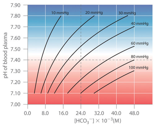
\[pH=6.10+\log \left( \dfrac{ [\ce{HCO3^{−}}]}{(3.0 \times 10^{−5} M/mm \;Hg)\; (P_{\ce{CO2}}) } \right) \label{Eq15} \]
Thus the pH of the solution depends on both the \(\ce{CO2}\) pressure over the solution and \([\ce{HCO3^{−}}]\). Figure \(\PageIndex{4}\) plots the relationship between pH and \([\ce{HCO3^{−}}]\) under physiological conditions for several different values of \(P_{\ce{CO2}}\), with normal pH and \([\ce{HCO3^{−}}]\) values indicated by the dashed lines.
According to Equation \ref{Eq15}, adding a strong acid to the \(\ce{CO2}/\ce{HCO3^{−}}\) system causes \([\ce{HCO3^{−}}]\) to decrease as \(\ce{HCO3^{−}}\) is converted to \(\ce{CO2}\). Excess \(\ce{CO2}\) is released in the lungs and exhaled into the atmosphere, however, so there is essentially no change in \(P_{\ce{CO2}}\). Because the change in \([\ce{HCO3^{−}}]/P_{CO_2}\) is small, Equation \ref{Eq15} predicts that the change in pH will also be rather small. Conversely, if a strong base is added, the \(\ce{OH^{-}}\) reacts with \(\ce{CO2}\) to form \(\ce{HCO3^{−}}\), but \(\ce{CO2}\) is replenished by the body, again limiting the change in both \([\ce{HCO3^{−}}]/P_{\ce{CO2}}\) and pH. The \(\ce{CO2}/\ce{HCO3^{−}}\) buffer system is an example of an open system, in which the total concentration of the components of the buffer change to keep the pH at a nearly constant value.
If a passenger steps out of an airplane in Denver, Colorado, for example, the lower \(P_{\ce{CO2}}\) at higher elevations (typically 31 mmHg at an elevation of 2000 m versus 40 mmHg at sea level) causes a shift to a new pH and \([\ce{HCO3^{-}}]\). The increase in pH and decrease in \([\ce{HCO3^{−}}]\) in response to the decrease in \(P_{\ce{CO2}}\) are responsible for the general malaise that many people experience at high altitudes. If their blood pH does not adjust rapidly, the condition can develop into the life-threatening phenomenon known as altitude sickness.
A Video Summary of the pH Curve for a Strong Acid/Strong Base Titration:
Summary of the pH Curve for a Strong Acid/Strong Base Titration(opens in new window) [youtu.be]
Summary
Buffers are solutions that resist a change in pH after adding an acid or a base. Buffers contain a weak acid (\(HA\)) and its conjugate weak base (\(A^−\)). Adding a strong electrolyte that contains one ion in common with a reaction system that is at equilibrium shifts the equilibrium in such a way as to reduce the concentration of the common ion. The shift in equilibrium is called the common ion effect. Buffers are characterized by their pH range and buffer capacity. The useful pH range of a buffer depends strongly on the chemical properties of the conjugate weak acid–base pair used to prepare the buffer (the \(K_a\) or \(K_b\)), whereas its buffer capacity depends solely on the concentrations of the species in the solution. The pH of a buffer can be calculated using the Henderson-Hasselbalch approximation, which is valid for solutions whose concentrations are at least 100 times greater than their \(K_a\) values. Because no single buffer system can effectively maintain a constant pH value over the physiological range of approximately 5 to 7.4, biochemical systems use a set of buffers with overlapping ranges. The most important of these is the \(CO_2/HCO_3^−\) system, which dominates the buffering action of blood plasma.