Lini Kinetics

Chemical kinetics deals with the rates of reactions. In order for a reaction to occur, a collision must occur; the collision must be of sufficient energy to break the necessary bonds and be of proper orientation. This is the basis of reaction rates. Factors effecting reaction rates are concentration of the reacting species found in the rate law, temperature and the presence or absence of a catalyst.

This section will discuss the determination of a rate law from experimental data and the effect of temperature on reaction rates.

A rate law of a reaction is a mathematical expression relating the rate of a reaction to the concentration of either reactants or products. One may not look at an overall reaction, and determine the rate law. The rate law may be theoretically determined from the rate determining step (slow step) of the reaction mechanism. Many chemical reactions actually require a number of steps in order to break bonds and form new ones. These series of steps are called the reaction mechanism. Reaction mechanisms are not typically covered in introductory level courses. The rate law of a reaction must be proven experimentally by looking at either the appearance of products or disappearance of reactants.

Consider the following overall chemical reaction:

\(\ce{2 NO(g) + O2(g) \rightleftharpoons 2 NO2(g)}\)

Here is an example of a rate law for the above reaction:

\(\mathrm{Rate = k[NO]^2[O_2]}\)

In this rate law, the rate of disappearance of \(\ce{NO}\) and \(\ce{O2}\) is proportional to the concentrations of \(\ce{NO}\) and \(\ce{O2}\), where \(\ce{k}\) is a rate constant (a proportionality constant). The exponents associated with each concentration term are referred to as the partial order. The sum of the partial orders gives the overall order of the reaction. In the above rate law, the partial order for \(\ce{NO}\) is 2 and is often referred to as 2^nd order. The partial order for \(\ce{O2}\) is 1 and is often refereed to as 1^st order. The overall order is 3 (3^rd order). It is important to note that the coefficients found in the balanced equation are not related to the exponents found in the rate law.

Let's look at a set of experimental data from which the rate law may be deduced. In this case, we will consider examining the rate in terms of the disappearance of reactants.

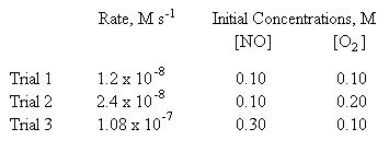
Experimentally one compiles the reaction rates relative to initial concentrations of reactants:

To determine the rate law, begin by examining the experimental data. Pick two trials to compare in which the concentration of one reactant is doubled while the concentration of the other reactant is held constant. We will be determining the partial order for the reactant whose concentration has changed. By keeping the concentration of the other reactant constant, we insure that the rate will not be affected by that reactant.

Let's begin by choosing the results for Trial 1 and Trial 2. In these two trials the concentration of \(\ce{NO}\) is held constant while the concentration of \(\ce{O2}\) has been doubled. To determine the partial order of \(\ce{O2}\), note that doubling the concentration of \(\ce{O2}\) also doubles the rate of the reaction. This may be mathematically expressed as:

For the equality to hold true, x must equal 1. This makes the partial order for \(\ce{O2}\) first order.

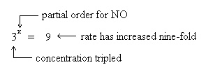
The same procedure is used to determine the partial order of \(\ce{NO}\). Pick two trials in which the concentration of \(\ce{O2}\) is held constant while the concentration of \(\ce{NO}\) is varied. These criteria are met with Trial 1 and Trial 3. The concentration of \(\ce{O2}\) is held constant while the concentration of \(\ce{NO}\) has tripled. Under these conditions, the rate of the reaction is increased nine fold. This may be expressed mathematically as:

For the equality to hold true, x must be 2. This makes the partial order for \(\ce{NO}\) second order. We are now able to write the rate law: \(\mathrm{Rate = k[NO]^2[O_2]}\), where \(\ce{k}\) is the rate constant. To solve for the rate constant, choose any experimental trial, and substitute for the rate, and concentrations of \(\ce{NO}\) and \(\ce{O2}\). Trial 1 data will be arbitrarily chosen in this case:

Thus the rate law becomes:

\(\mathrm{Rate = 1.2 \times 10^{-5}\, M^{-2}\, s^{-1}[NO]^2[O_2]}\)

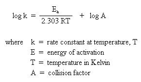
Another type of problem often encountered in kinetics involves the determination of the energy of activation for a chemical process. In order for a reaction to occur, a collision must take place. During this collision, existing bonds break and new bonds form. It takes energy to break bonds and energy is released when new bonds form. The collision must be of sufficient energy to break the necessary bonds. The energy source comes from the kinetic energy of the compound due to the velocity at which it is zipping around. Recall that the kinetic energy is temperature dependent. The higher the temperature, the faster the molecules are moving around, the greater the kinetic energy. This energy, as a function of kinetic energy and temperature, is called the energy of activation. The collision must also be of proper orientation. This is related by the collision factor. The combination of these aspects of the reaction are related to the rate of the reaction. Not all collisions are successful. These factors are related by a mathematical expression called the Arrhenius equation:

If one were to graph experimental data where \(\mathrm{\log k}\) is along the y-axis and \(\mathrm{\dfrac{1}{T}}\) is along the x-axis, a straight line would result. The slope of the line is \(\mathrm{\dfrac{E_a}{2.303R}}\), and the y-intercept corresponds to \(\mathrm{\log A}\). By determining the slope of the line mathematically, one could calculate the energy of activation. Similarly, if one extrapolates the line to the y-intercept, one could calculate the collision factor.

Since the slope embodies the energy of activation, a simplified form the Arrhenius equation could be used to determine the energy of activation. One requires knowledge of the rate constants at two different temperatures. Recall that the slope of a line is determined by the change in y over the change in x ("rise" over "run"). With this in mind, one is able to generate the following equation:

Since the y-intercept, \(\mathrm{\log A}\), is not part of the slope, it can be ignored. This equation may be used to solve the following problem:

A rate of reaction for a chemical process is investigated at two different temperatures. The rate of a reaction at 25 ^oC is 1.55 x 10^-4 s^-1. At 50 ^oC the rate of reaction is 3.88 x 10^-4 s^-1. Based on this data, what is the energy of activation for the chemical process expressed in J/mol?

To begin the problem, look at the units of the quantities given in the problem. The units for rate, s^-1, will cancel. Since the energy of activation is to be expressed in J/mol, the logical choice of the gas constant, \(\ce{R}\), will be 8.314 J/mol K. This choice of \(\ce{R}\) will dictate the units for temperature. Since the \(\ce{R}\) constant has temperature units expressed in kelvin, K, the temperatures given in the problem must be converted in kelvin as well. To convert from Celsius temperature units to kelvin units, add 273 to the Celsius temperature:

\(\mathrm{T_1 = 25 ^\circ C + 273 = 298\, K}\)

\(\mathrm{T_2 = 50^\circ C + 273 = 323\, K}\)

Substitute the rate constants and temperatures into the Arrhenius equation:

Solve for E_a. Remember to do the arithmetic inside the parenthesis first.

\(\mathrm{0.398 = (1.36 \times 10^{-5} \, mol/J) E_a}\)

\(\mathrm{E_a = \dfrac{0.398}{1.36 \times 10^{-5} \, mol/J} = 2.93 \times 10^4\, J/mol}\)