10.25: Boiling-Point Elevation and Freezing-Point Depression

We often encounter solutions in which the solute has such a low vapor pressure as to be negligible. In such cases the vapor above the solution consists only of solvent molecules and the vapor pressure is always lower than that of the pure solvent. Consider, for example, the solution obtained by dissolving 0.020 mol sucrose (C₁₂H₂₂O₁₁) in 0.980 mol H₂O at 100°C. The sucrose will contribute nothing to the vapor pressure, while we can expect the water vapor, by Raoult’s law, to contribute

\[P_{\text{H}_2 \text{O}}=P^*_{\text{H}_2\text{O}} * x_{ \text{H}_2 \text{O}} = 760 \text{mmHg} * 0.980 = 744.8 \text{mmHg} \nonumber \]

We would thus expect the vapor pressure to be 744.8 mmHg, in reasonable agreement with the observed value of 743.3 mmHg.

A direct consequence of the lowering of the vapor pressure by a nonvolatile solute is an increase in the boiling point of the solution relative to that of the solvent. We can see why this is so by again using the sucrose solution as an example. At 100°C this solution has a vapor pressure which is lower than atmospheric pressure, and therefore it will not boil. In order to increase the vapor pressure from 743.3 to 760 mmHg so that boiling will occur, we need to raise the temperature. Experimentally we find that the temperature must be raised to 100.56°C. We say that the boiling-point elevation ΔT_b is 0.56 K.

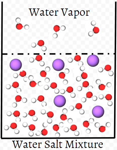
The image below demonstrates a solute dissolved in water. As you can see in the image, the presence of the solute interferes with the ability of the water to "escape" into the gaseous phase. This interference can be physical (as seen in the oversimplified image above) or it can be due to more complex factors, like intermolecular forces. Therefore, the solution has a lower vapor pressure for any given temperature. Thus, the mixture will require a higher temperature overall than a pure solution in order to boil, which is evident as a higher boiling boiling point.

A second result of the lowering of the vapor pressure is a depression of the freezing point of the solution. Any aqueous solution of a nonvolatile solute, for example, will have a vapor pressure at 0°C which is less than the vapor pressure of ice (0.006 atm or 4.6 mmHg) at this temperature. Accordingly, ice and the aqueous solution will not be in equilibrium. If the temperature is lowered, though, the vapor pressure of the ice decreases more rapidly than that of the solution and a temperature is soon reached when both ice and the solution have the same vapor pressure. Since both phases are now in equilibrium, this lower temperature is also the freezing point of the solution. In the case of the sucrose solution of mole fraction 0.02 described above, we find experimentally that the freezing point is –2.02°C.

We say that the freezing-point depression ΔT_f is 2.02 K.

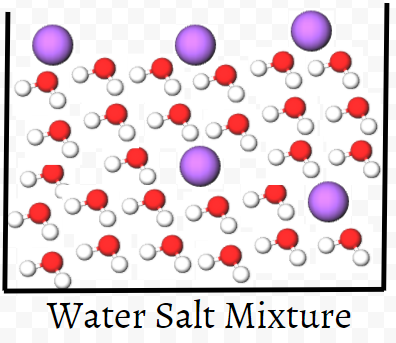
The image below demonstrates how this freezing point depression works on a very simple level. The salt (purple) in the water prevents the rigid, ordered arrangement of a solid from being achieved. The particles of solute block the crystallization of water, at least up until a certain point, causing a depression in the freezing point of the water.

The depression of the freezing point of water by a solute explains why the sea does not freeze at 0°C. Because of its high salt content the sea has a freezing point of –2.2°C. If the sea froze at 0°C, larger stretches of ocean would turn into ice and the climate of the earth would be very different. We can now also understand why we add ethylene glycol, CH₂OHCH₂OH, to water in a car radiator in winter. Without any additive the water would freeze at 0°C and the resulting increase in volume would crack the radiator. Since ethylene glycol is very soluble in water, it can form a solution with a freezing point low enough to prevent freezing even on the coldest winter day. Both the freezing-point depression and the boiling-point elevation of a solution were once important methods for determining the molar mass of a newly prepared compound. Nowadays a mass spectrometer is usually used for this purpose, often on an assembly-line basis. Many chemists send samples of newly prepared compounds to a laboratory specializing in these determinations in much the same way as a medical doctor will send a sample of your blood to a laboratory for analysis.

Note

The reason we can use the boiling-point elevation and the freezing-point depression to determine the molar mass of the solute is that both properties are proportional to the mole fraction and independent of the nature of the solute. The actual relationship, which we will not derive, is

\[x_{A}=\frac{\Delta H_{m}}{RT^{\text{2}}}\text{ }\Delta T \nonumber \]

where x_A is the mole fraction of the solute and ΔT is the boiling-point elevation or freezing-point depression. T indicates either the boiling point or freezing point of the pure solvent, and ΔH_m is the molar enthalpy of vaporization or fusion, whichever is appropriate. This relationship tells us that we can measure the mole fraction of the solute in a solution merely by finding its boiling point or freezing point of the solution.

Example \(\PageIndex{1}\): Mole Fraction

A solution of sucrose in water boils at 100.56°C and freezes at –2.02°C. Calculate the mole fraction of the solution from each temperature.

Solution

a) For boiling we have, from the Table of Molar Enthalpies of Fusion and Vaporization,

\[\triangle H_m = 40.7 \dfrac{\text{kJ}}{\text{mol}} \nonumber \] and \(T=373.15 \text{K}\)

As in previous examples the units of R should be compatible with the other units appearing in the equation. In this case since ΔH_m is given in units of kJ mol^–1, R = 8.314 J K^–1 mol^–1 is most appropriate. Since ΔT = 0.56 K, we have

\[x_{\text{sucrose}}=\frac{\Delta H_{m}}{RT^{\text{2}}}\Delta T=\frac{\text{40}\text{.7 }\times \text{ 10}^{\text{3}}\text{ J mol}^{-\text{1}}\text{ }\times \text{ 0}\text{.56 K}}{\text{8}\text{.314 J K}^{-\text{1}}\text{ mol}^{-\text{1}}\text{ (373}\text{.15)}^{\text{2}}}=\text{0}\text{.0197} \nonumber \]

b) Similarly for freezing we have

\[\triangle H_m = 6.01 \dfrac{kJ}{mol} \nonumber \] \(T=273.15 \text{K}\) \(\triangle T = 2.02 \text{K}\)

so that

\[x_{\text{sucrose}}=\dfrac{\text{6}\text{.01 }\times \text{ 10}^{\text{3}}\text{ J mol}^{-\text{1}}\text{ }\times \text{ 2}\text{.02 K}}{\text{8}\text{.314 J K}^{-\text{1}}\text{ mol}^{-\text{1}}\text{ }\times \text{ (273}\text{.15 K)}^{\text{2}}}=\text{0}\text{.0196} \nonumber \]

The two values are in reasonable agreement.

Once we know the mole fraction of the solute, its molar mass is easily calculated from the mass composition of the solution. 

Example \(\PageIndex{2}\): Molar Mass

33.07 g sucrose is dissolved in 85.27 g H₂O. The resulting solution freezes at –2.02°C. Calculate the molar mass of sucrose.

Solution

Since the freezing point of the solution is the same as in part b of Example 1, the mole fraction must be the same. Thus

\[x_{\text{sucrose}}=\text{0}\text{.0196}=\dfrac{n_{\text{sucrose}}}{n_{\text{sucrose}}\text{ + }n_{\text{H}_{\text{2}}\text{O}}} \nonumber \]

Furthermore \[\text{ }n_{\text{H}_{\text{2}}\text{O}}=\dfrac{\text{85}\text{.27 g}}{\text{18}\text{.02 g mol}^{-\text{1}}}=\text{4}\text{.732 mol} \nonumber \]

Thus \[\text{0}\text{.0196}=\dfrac{n_{\text{sucrose}}}{n_{\text{sucrose}}\text{ + 4}\text{.732 mol}} \nonumber \]

so that \[\begin{align} & \text{4}\text{.732 }\times \text{ 0}\text{.0196 mol}=n_{\text{sucrose}}-\text{0}\text{.0196}n_{\text{sucrose}} \\ & \text{ 0}\text{.092 75 mol}=\text{0}\text{.9804}n_{\text{sucrose}} \\ \end{align} \nonumber \] or \[\text{ }n_{\text{sucrose}}=\dfrac{\text{0}\text{.092 75}}{\text{0}\text{.9804}}\text{mol}=\text{0}\text{.0946 mol} \nonumber \]

From which \[\text{ }M_{\text{sucrose}}=\dfrac{\text{33}\text{.07 g}}{\text{0}\text{.0946 mol}}=\text{350 g mol}^{-\text{1}} \nonumber \]

Note: The correct molar mass is 342.3 g mol^–1. Neither the freezing point nor the boiling point gives a very accurate value for the molar mass of the solute.