9.3: Polymer Elasticity and Force–Extension Behavior

The Entropic Spring

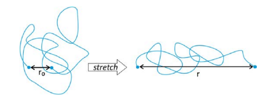
To extend a polymer requires work. We calculate the reversible work to extend the macromolecule from the difference in free energy of the chain held between the initial and final state. This is naturally related to the free energy of the system as a function of polymer end-to-end distance:

\[w_{stretch} = F(r) - F(r_0) = - \int_{r_0}^{r} \vec{f_{rev}} \cdot d \vec{r} \nonumber\]

For an ideal chain, the free energy depends only on the entropy of the chain: \(F = -TS\). There are fewer configurational states available to the chain as you stretch to larger extension. The number of configurational states available to the system can be obtained by calculating the conformational partition function, \(Q_{conf}\). For stretching in one-dimension, the Helmholtz free energy is:

\[\begin{array} {rcl} {dF} & = & {-pdV - SdT + f\cdot dx} \\ {} & = & {-k_B T \ln Q_{conf}} \\ {S_{conf}} & = & {k_B \ln Q_{conf}} \end{array}\nonumber\]

\[f = - \left (\dfrac{\partial F}{\partial x} \right )_{V, T, N} = -k_B T \dfrac{\partial \ln Q_{conf}}{\partial x} = -T \dfrac{\partial S_{conf}}{\partial x} \label{eq9.3.1}\]

When you increase the end-to-end distance, the number of configurational states available to the system decreases. This requires an increasingly high force as the extension approaches the contour length. Note that more force is needed to stretch the chain at higher temperature.

Since this is a freely joined chain and all microstates have the same energy, we can equate the conformational partition function of a chain at a particular extension \(x\) with the probability density for the end-to-end distances of that chain

\[Q_{conf} \to P_{fjc} (r)\nonumber\]

Although we are holding the ends of the chain at a fixed and stretching with the ends restrained along one direction (\(x\)), the probability distribution function takes the three-dimensional form to properly account for all chain configurations: \(P_{conf} (r) = P_0 e^{-\beta^2 r^2}\) with \(\beta^2 = 3k_B T/2n \ell^2\) and \(P_0 = \beta^3/\pi^{3/2}\) is a constant. Then

\[\ln P_{conf} (r) = -\beta^2 r^2 + \ln P_0 \nonumber\]

The force needed to extend the chain can be calculated from eq. (\(\ref{eq9.3.1}\)) after substituting \(r^2 = x^2 + y^2 + z^2\), which gives

\[f = -2\beta^2 k_B Tx = -\kappa_{st} x\nonumber\]

So we have a linear relationship between force and displacement, which is classic Hooke’s Law spring with a force constant \(\kappa_{st}\) given by

\[\kappa_{st} = \dfrac{3k_B T}{n\ell^2} = \dfrac{3k_B T}{\langle r^2 \rangle_0} \nonumber\]

Here \(\langle r^2 \rangle_0\) refers to the mean square end-to-end distance for the FJC in the absence of any applied forces. Remember: \(\langle r^2 \rangle_0 = n \ell^2 = \ell L_C\). In the case that all of the restoring force is due to entropy, then we call this an entropic spring \(\kappa_{ES}\).

\[\kappa_{ES} = \dfrac{T}{2} \left (\dfrac{\partial^2 S}{\partial x^2} \right )_{N, V, T}\nonumber\]

This works for small forces, while the force is reversible. Notice that \(\kappa_{ES}\) increases with temperature -- as should be expected for entropic restoring forces.

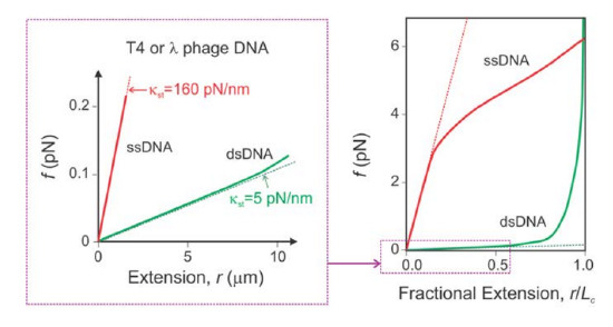
Example: Stretching DNA¹

At low force:

dsDNA \(\to \kappa_{st} = 5\ pN/nm\)

ssDNA \(\to \kappa_{st} = 160\ pN/nm \to \text{more entropy/more force}\)

At higher extension you asymptotically approach the contour length.

Force/Extension of a Random Walk Polymer

Let’s derive force extension behavior for a random walk polymer in one dimension. The end-to-end distance is \(r\), the segment length is \(r\), and the total number of segments is \(n\).

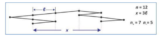
For any given \(r\), the number of configurations available to the polymer is:

\[\Omega = \dfrac{n!}{n_+ ! n_- !}\nonumber\]

This follows from recognizing that the extension of a random walk chain in one dimension is related to the difference between the number of segments that step in the positive direction, \(n_+\), and those that step in the negative direction, \(n_-\). The total number of steps is \(n = n_+ + n_-\). Also, the end-to-end distance can be expressed as

\[r = (n_+ - n_-) \ell = (2n_+ - n) \ell = (n - 2n_-) \ell \label{eq9.3.2}\]

\[n_{\pm} = \dfrac{1}{2} \left (n \pm \dfrac{r}{\ell} \right ) \ \ \ \ \ \ \dfrac{\partial n_{\pm}}{\partial r} = \pm \dfrac{1}{2\ell}\nonumber\]

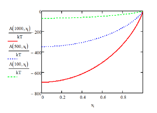
Then we can calculate the free energy of the random walk chain that results from the entropy of the chain, i.e., the degeneracy of configurational states at any extension. This looks like an entropy of mixing calculation:

\[\begin{array} {rcl} {F} & = & {-k_B T \ln \Omega} \\ {} & = & {-k_B T (n \ln n - n_+ \ln n_+ - n_- \ln n_-)} \\ {} & = & {nk_B T (\phi_+ \ln \phi_+ + \phi_- \ln \phi_-)} \end{array} \nonumber\]

\[\phi_{\pm} = \dfrac{n_{\pm}}{n} = \dfrac{1}{2} (1 \pm x)\nonumber\]

Here the fractional end-to-end extension of the chain is

\[x = \dfrac{r}{L_C}\]

Next we can calculate the force needed to extend the polymer as a function of \(r\):

\[f = -\dfrac{\partial F}{\partial r} \to \dfrac{\partial F}{\partial \phi_{\pm}} \dfrac{\partial \phi_{\pm}}{\partial r} \ \ \ \ \ \ \dfrac{\partial \phi_{\pm}}{\partial r} = \pm \dfrac{1}{2L_C} \nonumber\]

Using eq. (\(\ref{eq9.3.2}\))

\[\begin{array} {rcl} {f} & = & {-nk_B T (\ln \phi_+ - \ln \phi_-) \left (\dfrac{1}{2L_C} \right )} \\ {} & = & {-\dfrac{nk_B T}{2L_C} \ln \left (\dfrac{1 + x}{1 - x} \right )} \\ {} & = & {-\dfrac{k_B T}{\ell} \dfrac{1}{2} \ln \left (\dfrac{1 + x}{1 - x} \right )} \end{array}\nonumber\]

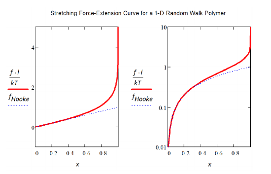
\[f = -\dfrac{k_B T}{\ell} \text{tanh}^{-1} (x) \label{eq9.3.4}\]

where \(I\) used the relationship: \(\ln \left (\dfrac{1 + x}{1 - x} \right ) = 2 \text{tanh}^{-1} (x)\). Note, here the forces are scaled in units of \(k_B T/\ell\). For small forces \(x \ll 1\), \(\text{tanh}^{-1} (x) \approx x\) and eq. (\(\ref{eq9.3.4}\)) gives \(f \approx \dfrac{k_B T}{\ell L_C} r\). This gives Hooke’s Law behavior with the entropic force constant expected for a 1D chain. For a 3D chain, we would expect: \(f \approx \dfrac{3k_B T}{\ell L_C} r\). The spring constant scales with dimensionality.

The relationship between position, force, and the partition function

Now let's do this a little more carefully. From classical statistical mechanics, the partition function is

\[Q = \int \int dr^{3N} dp^{3N} \exp (-H/k_B T)\nonumber\]

Where \(H\) is the Hamiltonian for the system. The average value for the position of a particle described by the Hamiltonian is

\[\langle x \rangle = \dfrac{1}{Q} \int \int dr^3 dp^3 x \exp (-H/k_B T)\nonumber\]

If the Hamiltonian takes the form

\[H = -f \cdot x \nonumber\]

Then

\[\langle x \rangle = \dfrac{k_B T}{Q} \left (\dfrac{\partial Q}{\partial f} \right )_{V, T, N} = k_B T \left (\dfrac{\partial \ln Q}{\partial f} \right )_{V, T, N} \nonumber\]

This describes the average extension of a chain if a force is applied to the ends.

Force/Extension Behavior for a Freely Jointed Chain

Making use of the expressions above and \(Q = q^N\)

\[q_{conf} = \int \int dr^3 dp^3 e^{-U/kT} e^{\vec{f} \cdot \vec{r}/k_B T} \ \ \ \ \ \ \ \langle r \rangle = Nk_B T \left (\dfrac{\partial \ln q_{conf}}{\partial f} \right )_{U, r, n}\nonumber\]

Here we also inserted a general Hamiltonian which accounts for the internal chain interaction potential and the force ex the chain: \(H = U - \vec{f} \cdot \vec{r}\). For \(N\) freely jointed chains with n segments, we set \(U \to 0\), and focus on force exerted on every segment of the chain.

\[\vec{f} \cdot \vec{r} = \sum_{i = 1}^{n} \vec{f} \cdot \vec{\ell_i} = f \ell \sum_{i = 1}^{n} \cos \theta_i\nonumber\]

Treating the segments as independent and integrating over all \(\theta\), we find that

\[q_{conf} (f) = \dfrac{2\pi \text{sinh} \varphi}{\varphi} \nonumber\]

\[\langle r \rangle = n \ell \left [\text{coth} \varphi - \dfrac{1}{\varphi} \right ] \]

where the unitless force parameter is

\[\varphi = \dfrac{f \ell}{k_B T}\]

As before, the magnitude of force is expressed relative to \(k_B T/\ell\). Note this calculation is for the average extension that results from a fixed force. If we want the force needed for a given average extension, then we need to invert the expression. Note, the functional form of the force-extension curve in eq. is different than what we found for the 1D random walk in eq. (\(\ref{eq9.3.4}\)). We do not expect the same form for these problems, since our random walk example was on a square lattice, and the FJC propagates radially in all directions.

Derivation

For a single polymer chain:

\[\begin{array} {rcl} {q} & = & {\int \int dr^3 dp^3 e^{U/k_B T} e^{-f \cdot r/k_B T}} \\ {P(r)} & = & {\dfrac{1}{q} e^{-U/k_B T} e^{f \cdot r/k_B T}} \\ {\langle r \rangle} & = & {\dfrac{k_B T}{q} \left (\dfrac{\partial \ln q}{\partial f} \right )_u} \end{array}\nonumber\]

In the case of the Freely Jointed Chain, set \(U \to 0\).

\[\vec{f} \cdot \vec{r} = \vec{f} \cdot \sum_{i =1}^{n} \vec{\ell_i} = f \ell \sum_{i = 1}^{n} \cos \theta_i \nonumber\]

Decoupled segments:

\[\begin{array} {rcl} {q} & \approx & {\int dr^3 \exp \left (\sum_i \dfrac{f \ell}{k_B T} \cos \theta_i \right )} \\ {} & = & {(\int_{0}^{2\pi} \int_{0}^{\pi} \exp [\varphi \cos \theta] \sin \theta d \theta d \phi)^n} \\ {} & = & {\left (\dfrac{2\pi \text{sinh} (\varphi)}{\varphi} \right )^n} \\ {\langle r \rangle} & = & {k_B T \dfrac{\partial}{\partial f} \ln q} \\ {} & = & {nk_B T \dfrac{\partial}{\partial f} \left [\ln \left \{\dfrac{2\pi \text{sinh} (\varphi)}{\varphi} \right \} \right ] \ \ \ \ \ \ \text{coth} (x) = \dfrac{e^x + e^{-x}}{e^x - e^{-x}}} \\ {\langle r \rangle} & = & {n \ell [\text{coth} (\varphi) - \varphi^{-1}]} \\ {\text{or } \langle x \rangle = \text{coth} (\varphi) - \varphi^{-1}} & \ & {\text{ The average fractional extension: } \langle x \rangle = \langle r \rangle / L_C} \end{array} \nonumber\]

Now let’s look at the behavior of the expression for \(\langle x \rangle\) -- also known as the Langevin function.

\[\langle r \rangle = n \ell [\text{coth} (\varphi) - \varphi^{-1}]\]

Looking at limits:

• Weak force \((\varphi \ll 1): f \ll k_B T/\ell\)
  Inserting and truncating the expansion: \(\text{coth} \varphi = \dfrac{1}{\varphi} + \dfrac{1}{3} \varphi - \dfrac{1}{45} \varphi^3 + \dfrac{2}{945} \varphi^5 + \cdots\), we get
  \[\begin{array} {rcl} {\langle x \rangle} & = & {\dfrac{\langle r \rangle}{L_C} \approx \dfrac{1}{3} \varphi} \\ {\langle r \rangle} & \approx & {\dfrac{1}{3} \dfrac{n \ell^2}{k_B T} f} \\ {\text{or } \ \ \ f} & = & {\dfrac{3k_B T}{n \ell^2} \langle r \rangle = \kappa_{ES} \langle r \rangle} \end{array} \nonumber\]
  Note that this limit has the expected linear relationship between force and displacement, which is governed by the entropic spring constant.
• Strong force (\(\varphi \gg 1\)). \(f \gg k_B T / \ell\) Taking the limit \(\text{coth} (x) \to 1\).
  \[\langle r \rangle \simeq n \ell \left [1 - \dfrac{1}{\varphi} \right ] \longleftarrow \lim_{f \to \infty} = \lim_{\alpha \to \infty} = L_C \text{ Contour length} \nonumber\]
  \[\text{Or } f = \dfrac{k_B T}{\ell} \dfrac{1}{1 - \langle x \rangle} \text{ where } \langle x \rangle = \dfrac{\langle r \rangle}{L_C} \nonumber\]
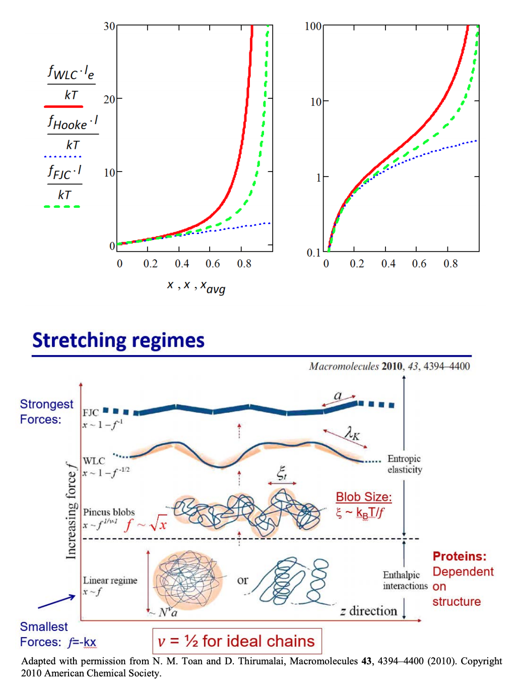
  For strong force limit, the force extension behavior scales as, \(x \sim 1 - f^{-1}\).

So, what is the work required to extend the chain?

At small forces, we can integrate over the linear force-extension behavior. Under those conditions, to extend from \(r\) to \(r+\Delta r\), we have

\[w_{rev} = \int_0^{\Delta r} \kappa_{ES} r dr = \dfrac{3k_B T}{2n \ell^2} \Delta r^2\nonumber\]

Force/Extension of Worm-like Chain

For the worm-like chain model, we found that the variance in the end-to-end distance was

\[\langle r^2 \rangle = 2 \ell_p L_C - 2 \ell_p^2 (1 - e^{-L_C/\ell_p}) \label{eq9.3.8}\]

where \(L_C\) is the contour length, and the persistence length was related to the bending force constant as \(\ell_p = \dfrac{\kappa_b}{k_B T}\). The limiting behavior for eq. (\(\ref{eq9.3.8}\)) is:

\[\begin{array} {lclcrclcl} {\text{rigid:}} & \ \ & {\ell_p \gg L_C} & \ \ & {\langle r^2 \rangle} & \propto & {L_C^2} & \ \ & {} \\ {\text{flexible:}} & \ \ & {\ell_p \ll L_C} & \ \ & {\langle r^2 \rangle} & \sim & {2L_C \ell_p} & \ \ & {\therefore \text{for WLC}} \\ {} & \ \ & {} & \ \ & {} & = & {n_e \ell_e^2} & \ \ & {(2 \ell_p = \ell_e)} \end{array} \nonumber\]

Following a similar approach to the FJC above, it is not possible to find an exact solution for the force-extension behavior of the WLC, but it is possible to show the force extension behavior in the rigid and flexible limits.

Setting \(2\ell_p = \ell_e\), \(\varphi = f\ell_e /k_B T\), and using the fractional extension \(\langle x \rangle = \dfrac{\langle r \rangle}{L_C}\):

1. Weak force (\(\varphi \ll 1\)) Expected Hooke’s Law behavior
   \[f \ell_e \ll k_B T \ \ \ \ \ \ \ \ \ \ f = \dfrac{3k_B T}{\ell_e L_C} \longrightarrow \dfrac{f \ell_e}{k_B T} = 3\langle x \rangle \nonumber\]
   For weak force limit, the force extension behavior scales as, \(x \sim f\).
2. Strong force (\(\varphi \gg 1\))
   \[f \ell_e \gg k_B T \ \ \ \ \ \ \ \ \langle r \rangle = L_C \left (1 - \dfrac{1}{2\sqrt{\varphi}} \right ) \longrightarrow \dfrac{f \ell_e}{k_B T} = \dfrac{1}{4(1 - \langle x \rangle)^2} \nonumber\]
   For strong force limit, the force extension behavior scales as, \(x \sim 1 - f^{-1/2}\).

An approximate expression for the combined result (from Bustamante):

\[\dfrac{f\ell_p}{kT} = \dfrac{1}{4(1 - \langle x \rangle)^2} - \dfrac{1}{4} + \langle x \rangle\]

_____________________________

1. A. M. van Oijen and J. J. Loparo, Single-molecule studies of the replisome, Annu. Rev. Biophys. 39, 429–448 (2010).