4.2: Solvation Thermodynamics

Let’s consider the thermodynamics of an aqueous solvation problem. This will help identify various physical processes that occur in solvation, and identify limitations to this approach. Solvation is described as the change in free energy to take the solute from a reference state, commonly taken to be the isolated solute in vacuum, into dilute aqueous solution:

Solute(\(g\)) \(\to\) Solute(\(aq\))

Conceptually, it is helpful to break this process into two steps: (1) the energy required to open a cavity in the liquid, and (2) the energy to put the solute into the cavity and turn on the interactions between solute and solvent.

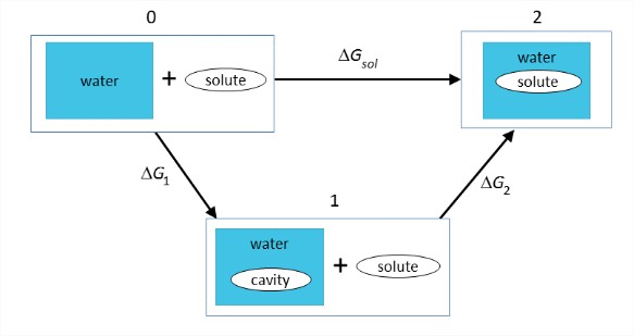
Each of these terms has enthalpic and entropic contributions:

\[\begin{array} {rcl} {\Delta G_{\text{sol}}} & = & {\Delta H_{\text{sol}} - T \Delta S_{\text{sol}}} \\ {\Delta G_{\text{sol}}} & = & {\Delta G_1 + \Delta G_2} \\ {} & = & {\Delta H_1 - T\Delta S_1 + \Delta H_2 - T \Delta S_2} \end{array} \nonumber\]

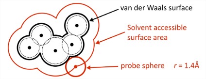
\(\Delta G_1\): Free energy to open a cavity in water. We are breaking the strong cohesive intermolecular interactions in water (\(\Delta H_1\)), creating a void against constant pressure, and reducing the configurational entropy of the water hydrogen-bond network (\(\Delta S_1\)). Therefore \(\Delta G_1\) is large and positive.The hydrophobic effect is dominated by this term. In atomistic models, cavities for biomolecules are commonly defined through the solute’s solvent accessible surface area (SASA). In order to account for excluded volume on the distance scale of a water molecule, the SASA can be obtained by rolling a sphere with radius 1.4 \(\mathring{A}\) over the solute’s van der Waals surface.

\(\Delta G_2\): Free energy to insert the solute into the cavity, turn on the interactions between solute and solvent. Ion and polar solvation is usually dominated by this term. This includes the favorable electrostatic and H-bond interactions (\(\Delta H_2\)). It also can include a restructuring of the solute and/or solvent at their interface due to the new charges. The simplest treatment of this process describes the solvent purely as a homogeneous dielectric medium and the solute as a simple sphere or cavity embedded with point charges or dipoles. It originated from the Born–Haber cycle first used to describe \(\Delta H_{rxn}\) of gas-phase ions, and formed the basis for numerous continuum and cavity-in-continuum approaches to solvation.

Given the large number of competing effects involving solute, solvent, and intermolecular interactions, predicting the outcome of this process is complicated.

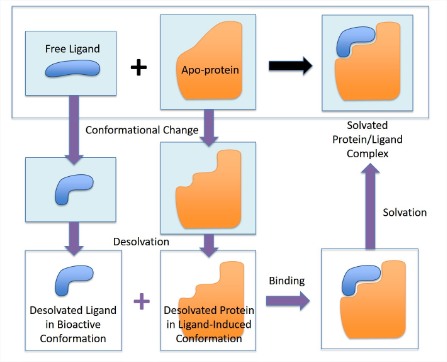
Looking at the cycle above illustrates many of the complications from this approach relevant to molecular biophysics, even without worrying about atomistic details. From a practical point of view, the two steps in this cycle can often have large magnitude but opposite sign, resulting in a high level of uncertainty about \(\Delta G_{\text{sol}}\)—even its sign! More importantly, this simplified cycle assumes that a clean boundary can be drawn between solute and solvent—the solvent accessible surface area. It also assumes that the influence of the solvent is perturbative, in the sense that the solvent does not influence the structure of the solute or that there is conformational disorder or flexibility in the solute and/or solvent. However, even more detailed thermodynamic cycles can be used to address some of these limitations:

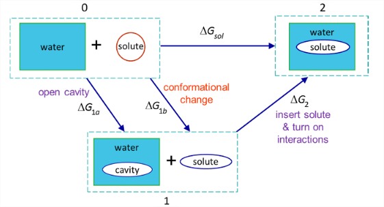
\(\Delta G_{1a}\): Free energy to create a cavity in water for the final solvated molecule.

\(\Delta G_{1b}\): Free energy to induce the conformational change to the solute for the final solvated state.

\(\Delta G_{2}\): Free energy to insert the solute into the cavity, turn on the interactions between solute and solvent. This includes turning on electrostatic interactions and hydrogen bonding, as well as allowing the solvent to reorganize around the solute:

\[\Delta G_{2} = \Delta G_{\text{solute-solvent}} + \Delta G_{\text{solvent reorg}}\nonumber\]

Configurational entropy may matter for each step in this cycle, and can be calculated using¹

\[S=-k_{B} \sum_{i} P_{i} \ln P_{i} \nonumber\]

Here sum is over microstate probabilities, which can be expressed in terms of the joint probability of the solute with a given conformation and the probability of a given solvent configuration around that solute structure. In step 1, one can average over the conformational entropy of the solvent for the shape of the cavity (1a) and the conformation of the solute (1b). Step 2 includes solvent configurational variation and the accompanying variation in interaction strength.

With a knowledge of solvation thermodynamics for different species, it becomes possible to construct thermodynamic cycles for a variety of related solvation processes:

1) Solubility. The equilibrium between the molecule in its solid form and in solution is quantified through the solubility product \(K_{sp}\), which depends on the free energy change of transferring between these phases

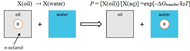
2) Transfer free energy. The most common empirical way of quantifying hydrophobicity is to measure the partitioning of a solute between oil and water. The partitioning coefficient \(P\) is related to the free energy needed to transfer a solute from the nonpolar solvent (typically octanol) to water

3) Bimolecular association processes

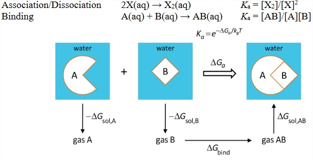
Binding with conformational selection

____________________________________________

1. See C. N. Nguyen, T. K. Young and M. K. Gilson, Grid inhomogeneous solvation theory: Hydration structure and thermodynamics of the miniature receptor cucurbit[7]uril, J. Chem. Phys. 137 (4), 044101 (2012).