1.2: Radial Distribution Function

"Structure" implies that the positioning of particles is regular and predictable. This is possible in a fluid to some degree when considering the short-range position and packing of particles. The local particle density variation should show some structure in a statistically averaged sense. Structure requires a reference point, and in the case of a fluid we choose a single particle as the reference and describe the positioning of other particles relative to that. Since each particle of a fluid experiences a different local environment, this information must be statistically averaged, which is our first example of a correlation function. For distances longer than a "correlation length", we should lose the ability to predict the relative position of a specific pair of particles. On this longer length scale, the fluid is homogeneous.

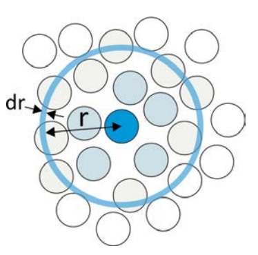
The radial distribution function, \(g(r)\), is the most useful measure of the "structure" of a fluid at molecular length scales. Although it invokes a continuum description, by "fluid" we mean any dense, disordered system which has local variation in the position of its constituent particles but is macroscopically isotropic. \(g(r)\) provides a statistical description of the local packing and particle density of the system, by describing the average distribution of particles around a central reference particle. We define the radial distribution function as the ratio of \(\langle \rho (r) \rangle \), the average local number density of particles at a distance \(r\), to the bulk density of particles, \(\rho \):

\[g(r) =\dfrac{\langle \rho (r) \rangle }{\rho}\nonumber\]

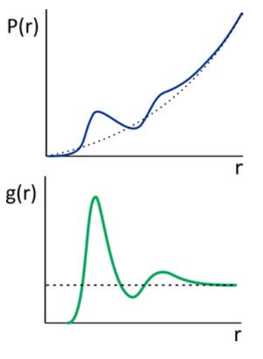
In a dense system, \(g(r)\) starts at zero (since it does not count the reference particle), rises to a peak at the distance characterizing the first shell of particles surrounding the reference particle (i.e., the \(1^{\text{st}}\) solvation shell), and approaches 1 for long distances in isotropic media. The probability of finding a particle at a distance \(r\) in a shell of thickness \(dr\) is \(P(r)=4 \pi r^{2} g(r)\ \mathrm{d} r\), so integrating \(\rho \cdot g(r)\) over the first peak in gives the average number of particles in the first shell.

The radial distribution function is most commonly used in gasses, liquids, and solutions, since it can be used to calculate thermodynamic properties such as the internal energy and pressure of the system. But is relevant at any size scale, such as packing of colloids, and is useful in complex heterogeneous media, such as the distribution of ions around DNA. For correlating the position of different types of particles, the radial distribution function is defined as the ratio of the local density of "\(b\)" particles at a distance \(r\) from "\(a\)" particles, \(g_{a b}(r)= \left \langle \rho_{ab}(r)\right \rangle /\rho \) In practice, \(\rho_{ab} (r)\) is calculated by looking radially from an "\(a\)" particle at a shell at distance \(r\) and of thickness \(\mathrm{d} r\), counting the number of "\(b\)" particles within that shell, and normalizing the count by the volume of that shell.

Two-Particle Density Correlation Function¹

Let’s look a little deeper, considering particles of the same type, as in an atomic liquid or granular material. If there are \(N\) particles in a volume \(V\), and the position of the \(i^{\text{th}}\) particle is \(\bar{r_i}\), then the number density describes the position of particles,

\[\rho(\bar{r})=\sum_{i=1}^{N} \delta \left (\bar{r} - \bar{r_i}\right) \nonumber\]

The average of a radially varying property given by \(X(r)\) is determined by

\[\langle X(r)\rangle=\dfrac{1}{V} \int_{V} X(r) 4 \pi r^{2} d r \nonumber\]

Integrating \(\rho(\bar{r})\) over a volume gives the particle number in that volume.

\[\int_{V} \rho(r) 4 \pi r^{2} d r=N \nonumber\]

When the integral is over the entire volume, we can use this to obtain the average particle density:

\[\dfrac{1}{V} \int_{0}^{\infty} \rho (r) 4 \pi r^{2} d r = \dfrac{N}{V} = \rho \nonumber\]

Next, we can consider the spatial correlations between two particles, \(i\) and \(j\). The two-particle density correlation function is

\[\rho \left(\bar{r}, \vec{r}' \right) = \left \langle \sum_{i=1}^{N} \delta \left( \bar{r}- \bar{r_i} \right) \sum_{j=1}^{N} \delta \left(\vec{r}'-\bar{r_j}\right) \right \rangle \nonumber\]

This describes the conditional probability of finding particle \(i\) at position \(r_i\) and particle \(j\) at position \(r_j\). We can expand and factor \(\rho (\bar{r}, \bar{r}')\) into two terms depending on whether \(i = j\) or \(i \ne j\):

\[\begin{array} {rcl} {\rho \left(\bar{r}, \vec{r}' \right)} & = & {N \left \langle \delta (\bar{r} - \bar{r_i}) \delta (\bar{r} - \bar{r_i}) \right \rangle + N(N - 1) \left \langle \delta (\bar{r} - \bar{r_i}) \delta (\bar{r}' - \bar{r_j}) \right \rangle} \\ {} & = & {\rho^{(1)} + \rho^{(2)} \left(\bar{r}, \vec{r}' \right)} \end{array}\nonumber\]

The first term describes the self-correlations, of which there are \(N\) terms: one for each atom.

\[\rho^{(1)}=N \left \langle \delta \left( \bar{r} - \bar{r_i} \right) \delta \left (\bar{r}' -\bar{r_i} \right ) \right \rangle = \rho \nonumber\]

The second term describes the two-body correlations, of which there are \(N(N‒1)\) terms.

\[\begin{array} {rcl} {\rho^{(2)} \left ( \bar{r}, \bar{r}' \right )} & = & {N(N - 1) \left \langle \delta (\bar{r} - \bar{r_i}) \delta (\bar{r}' - \bar{r_j}) \right \rangle } \\ {} & = & {\dfrac{N^2}{V^2} g \left ( \bar{r}, \bar{r}' \right ) = \rho^2 g \left ( \bar{r}, \bar{r}' \right )} \end{array} \nonumber\]

\(g() = \rho^{(2)} \left ( \bar{r}, \bar{r}' \right )/ \rho^2\) is the two-particle distribution function, which describes spatial correlation between two atoms or molecules. For isotropic media, it depends only on distance between particles, \(g \left ( \left | \bar{r}, \bar{r}' \right | \right ) = g(r)\), and is therefore also called the radial pair-distribution function.

We can generalize \(g(r)\) to a mixture of \(a\) and \(b\) particles by writing \(g_{ab} (r)\):

\[\begin{array} {c} {g_{ab} (r) = \dfrac{\rho_{ab}(r)}{N_{b} / V}} \\ {N_{b}=\int_{V} dr 4 \pi r^{2} \rho_{ab}(r)} \end{array}\nonumber\]

Potential of Mean Force

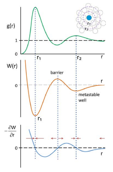
One can use \(g(r)\) to describe the free energy for bringing two particles together as

\[W(r)=-k_{B} T \ln g(r) \nonumber \]

\(W(r)\) is known as the potential of mean force. We are taking a free energy which is a function of many internal variables and projecting it onto a single coordinate. \(W(r)\) is a potential function that can be used to obtain the mean effective forces that a particle will experience at a given separation \(f = -\partial W /\partial r\).

_________________________________

1. J. P. Hansen and I. R. McDonald, Theory of Simple Liquids, \(2^{\text{nd}}\) Ed. (Academic Press, New York, 1986); D. A. McQuarrie, Statistical Mechanics. (Harper & Row, New York, 1976).