The Q-Test

Last updated
Save as PDF

Page ID: 276168

Contributor
Analytical Sciences Digital Library

\( \newcommand{\vecs}[1]{\overset { \scriptstyle \rightharpoonup} {\mathbf{#1}} } \) \( \newcommand{\vecd}[1]{\overset{-\!-\!\rightharpoonup}{\vphantom{a}\smash {#1}}} \)\(\newcommand{\id}{\mathrm{id}}\) \( \newcommand{\Span}{\mathrm{span}}\) \( \newcommand{\kernel}{\mathrm{null}\,}\) \( \newcommand{\range}{\mathrm{range}\,}\) \( \newcommand{\RealPart}{\mathrm{Re}}\) \( \newcommand{\ImaginaryPart}{\mathrm{Im}}\) \( \newcommand{\Argument}{\mathrm{Arg}}\) \( \newcommand{\norm}[1]{\| #1 \|}\) \( \newcommand{\inner}[2]{\langle #1, #2 \rangle}\) \( \newcommand{\Span}{\mathrm{span}}\) \(\newcommand{\id}{\mathrm{id}}\) \( \newcommand{\Span}{\mathrm{span}}\) \( \newcommand{\kernel}{\mathrm{null}\,}\) \( \newcommand{\range}{\mathrm{range}\,}\) \( \newcommand{\RealPart}{\mathrm{Re}}\) \( \newcommand{\ImaginaryPart}{\mathrm{Im}}\) \( \newcommand{\Argument}{\mathrm{Arg}}\) \( \newcommand{\norm}[1]{\| #1 \|}\) \( \newcommand{\inner}[2]{\langle #1, #2 \rangle}\) \( \newcommand{\Span}{\mathrm{span}}\)\(\newcommand{\AA}{\unicode[.8,0]{x212B}}\)

In earlier modules we introduced the idea of a normal distribution (the so-called "bell-shaped" curve)

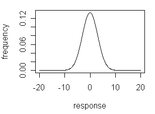
whose shape is symmetrical, and is centered on the population's mean with a width that is proportional to the population's standard deviation. We also learned that the probability of obtaining a particular response for any single sample is greatest when its value is close to the mean and smallest when its value is far from the mean. For example, there is a probability of only 0.15% that a single sample will have a value that is larger than the mean plus three standard deviations. It is unlikely, therefore, that the result for any replicate will be too far removed from the results of other replicates.

There are several ways for determining the probability that a result is an outlier. One of the most common approaches is called Dixon's Q-test. The basis of the Q-test is to compare the difference between the suspected outlier's value and the value of the result nearest to it (the gap) to the difference between the suspected outlier's value and the value of the result furthest from it the range).

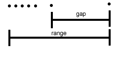
The value Q is defined as the ratio of the gap to the range

\[\mathrm{Q=\dfrac{gap}{range}}\nonumber\]

where both "gap" and "range" are positive. The larger the value of Q, the more likely that the suspected outlier does not belong to the same population as the other data points. The value of Q is compared to a critical value, Q_crit, at one of three common confidence levels: 90%, 95%, and 99%. For example, if we choose to work at the 95% confidence level and find that

\[\mathrm{Q ≤ Q_{crit}}\nonumber\]

then we cannot be 95% confident that the suspected outlier comes from a different population and we retain the data point. On the other hand, if

\[\mathrm{Q >Q_{crit}}\nonumber\]

then we can be at least 95% confident that the suspected outlier comes from a different population and can discard it. Of course, there also is as much as a 5% chance that this conclusion is incorrect.

Data that are more tightly clustered, as in this example,

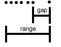
are less likely to yield a value for Q that favors the identification of an outlier.

When you are ready, proceed to Problem 1.