
Spectral Data Set with Suggested Uses
- Page ID
- 292501

\( \newcommand{\vecs}[1]{\overset { \scriptstyle \rightharpoonup} {\mathbf{#1}} } \)
\( \newcommand{\vecd}[1]{\overset{-\!-\!\rightharpoonup}{\vphantom{a}\smash {#1}}} \)
\( \newcommand{\id}{\mathrm{id}}\) \( \newcommand{\Span}{\mathrm{span}}\)
( \newcommand{\kernel}{\mathrm{null}\,}\) \( \newcommand{\range}{\mathrm{range}\,}\)
\( \newcommand{\RealPart}{\mathrm{Re}}\) \( \newcommand{\ImaginaryPart}{\mathrm{Im}}\)
\( \newcommand{\Argument}{\mathrm{Arg}}\) \( \newcommand{\norm}[1]{\| #1 \|}\)
\( \newcommand{\inner}[2]{\langle #1, #2 \rangle}\)
\( \newcommand{\Span}{\mathrm{span}}\)
\( \newcommand{\id}{\mathrm{id}}\)
\( \newcommand{\Span}{\mathrm{span}}\)
\( \newcommand{\kernel}{\mathrm{null}\,}\)
\( \newcommand{\range}{\mathrm{range}\,}\)
\( \newcommand{\RealPart}{\mathrm{Re}}\)
\( \newcommand{\ImaginaryPart}{\mathrm{Im}}\)
\( \newcommand{\Argument}{\mathrm{Arg}}\)
\( \newcommand{\norm}[1]{\| #1 \|}\)
\( \newcommand{\inner}[2]{\langle #1, #2 \rangle}\)
\( \newcommand{\Span}{\mathrm{span}}\) \( \newcommand{\AA}{\unicode[.8,0]{x212B}}\)
\( \newcommand{\vectorA}[1]{\vec{#1}} % arrow\)
\( \newcommand{\vectorAt}[1]{\vec{\text{#1}}} % arrow\)
\( \newcommand{\vectorB}[1]{\overset { \scriptstyle \rightharpoonup} {\mathbf{#1}} } \)
\( \newcommand{\vectorC}[1]{\textbf{#1}} \)
\( \newcommand{\vectorD}[1]{\overrightarrow{#1}} \)
\( \newcommand{\vectorDt}[1]{\overrightarrow{\text{#1}}} \)
\( \newcommand{\vectE}[1]{\overset{-\!-\!\rightharpoonup}{\vphantom{a}\smash{\mathbf {#1}}}} \)
\( \newcommand{\vecs}[1]{\overset { \scriptstyle \rightharpoonup} {\mathbf{#1}} } \)
\( \newcommand{\vecd}[1]{\overset{-\!-\!\rightharpoonup}{\vphantom{a}\smash {#1}}} \)
Using R to Introduce Students to Principal Component Analysis, Cluster Analysis, and Multiple Linear Regression
DAVID HARVEY
PITTCON 2018
Data Set
Filename: CuCoCrNi.xlsx
File Structure: visible spectra recorded at 642 wavelengths (380.5 nm – 899.5 nm) for 80 solutions that contain 1 – 4 of Cu2+, Co2+, Cr3+, or Ni2+ in 0.10 M HNO3, recorded using a Vernier SpectroVis Plus spectrometer using LoggerPro, and exported as a .csv file
- column a: id for sample
- column b: list of analytes in the sample
- column c: number of analytes in the sample (labeled as dimension)
- column d: concentration of Cu2+ (prepared from single stock solution of 0.0500 M Cu2+)
- column e: concentration of Co2+ (prepared from single stock solution of 0.100 M Co2+)
- column f: concentration of Cr3+ (prepared from single stock solution of 0.0375 M Cr2+)
- column g: concentration of Ni2+ (prepared from single stock solution of 0.130 M Ni2+)
- columns h – xr: absorbance at the stated wavelength
Suggested Uses:
- analysis for single analyte using external standards calibration
- multicomponent analysis of binary, ternary, and quaternary mixtures
- choosing wavelengths for Beer’s law analysis
- principal component analysis
- cluster analysis
- multiple linear regression
Context
Chem 351: Chemometrics
This course, Chem 351: Chemometrics, provides an introduction to how chemists and biochemists can extract useful information from the data they collect in lab, including, among other topics, how to summarize data, how to visualize data, how to test data, how to build quantitative models to explain data, how to design experiments, and how to separate a useful signal from noise.
Two 60 minute class periods per week for 14 weeks. Course is divided into 12 units.
- Unit 1: Introduction
- Unit 2: Basic Statistics
- Unit 3: Distribution of Data
- Unit 4: Confidence Intervals
- Unit 5: Analysis of Variance
- Unit 6: Linear Regression
- Unit 7: 3D Visualizations
- Unit 8: Experimental Design
- Unit 9: Signal Processing
- Unit 10: Principal Component Analysis
- Unit 11: Cluster Analysis
- Unit 12: Multiple Linear Regression
R as a Tool for Teaching Chemometrics
- data-centric programming language and environment for statistical computing
- large number of users ensures longevity of software
- base installation provides access to a wide variety of computational methods for processing data and tools for visualizing data
- highly extensible through user-written scripts and packages of functions
- available via Free Software Foundation’s GNU General Public License
- versions for UNIX, Linux, Windows, and MacOS platforms
- easy to interweave text, tables, and figures
- base packages are very stable so code is resilient
For further details regarding R, see https://www.r-project.org/
Note
Make R a tool, not a barrier. Emphasis is on adapting coding examples, using coding templates, using available packages, and using functions provided by instructor
The Analytical System: Beer’s Law
- stock standards
- 0.0500 M Cu2+
- 0.1000 M Co2+
- 0.0375 M Cr3+
- 0.1300 M Ni2+
- all in 0.10 M HNO3
- samples prepared from stocks
- single metal ions
- binary mixtures of metal ions
- ternary mixtures of metal ions
- quaternary mixtures of metal ions
- spectra collected with a Vernier SpectroVis Plus spectrometer; exported as .csv files
- individual .csv files combined into a single file, cleaned up, and saved as a .csv file.
- file has 80 rows (one per sample) and 642 columns (seven with information on composition of samples and absorbance values at 635 wavelengths).
- data set is brought into R using the readr package’s read_csv( ) function and then further subsetted within R to create individual data files.
Prelude
External Standardization for Copper
\[A_\textrm{λ,Cu} = ε_\textrm{λ,Cu}bC_\textrm{Cu}\nonumber\]
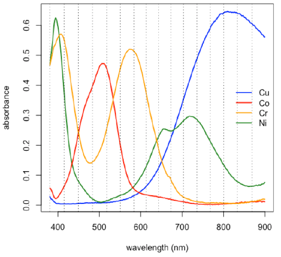
- plot spectra for set of standards and identify the wavelength of maximum absorbance
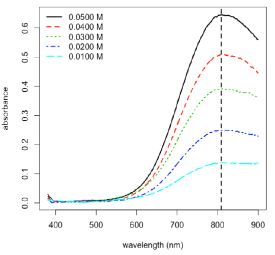
\[\mathrm{λ = 809.1\: nm}\nonumber\]
-
R functions: readr::read_csv( ), matplot( ), legend( ), which.max( ), abline( )
-
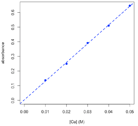
- plot calibration data and determine equation for calibration curve
Coefficients:
Estimate
Std. Error
t value
Pr(>|t|)
(Intercept)
0.003202
0.008222
0.389
0.723
cuStd_conc
12.778883
0.247900
51.548
1.61e-05 ***
---Signif. codes: 0 ‘***’ 0.001 ‘**’ 0.01 ‘*’ 0.05 ‘.’ 0.1 ‘ ’ 1 Residual standard error: 0.007839 on 3 degrees of freedom Multiple R-squared: 0.9989, Adjusted R-squared: 0.9985 F-statistic: 2657 on 1 and 3 DF, p-value: 1.608e-05 \[A = 12.78\: \textrm{M}^{–1} × C + 0.0032\nonumber\]
-
R functions: plot( ), lm( ), abline( ), summary( )
-
- determine concentration of copper in an unknown using the chemCal package
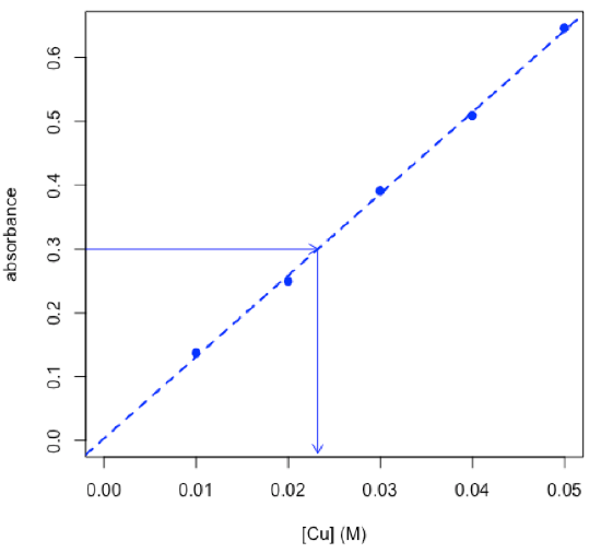
$Prediction[1] 0.02322567
$`Standard Error`[1] 0.0006847376
$Confidence[1] 0.002179141
$`Confidence Limits`[1] 0.02104653 0.02540481
\[C_\textrm{Cu} = \mathrm{0.0232\: M ± 0.0022\: M}\nonumber\]
-
R functions: chemCal::inverse.predict( ), arrows( )
-
Analysis of Binary Mixture: Cu and Ni
\[A_\textrm{λ1,mix} = ε_\textrm{λ1,Cu}bC_\textrm{Cu} + ε_\textrm{λ1,Ni}bC_\textrm{Ni}\nonumber\]
\[A_\textrm{λ2,mix} = ε_\textrm{λ2,Cu}bC_\textrm{Cu} + ε_\textrm{λ2,Ni}bC_\textrm{Ni}\nonumber\]
- plot spectra for a Cu standard, for a Ni standard, and for a mixture, and identify the wavelengths to use for the analysis
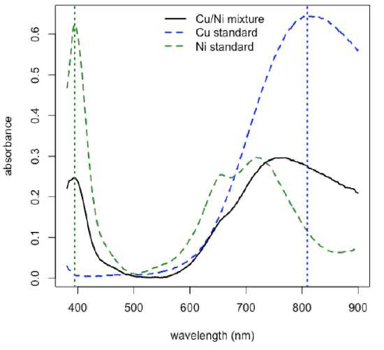
\[\mathrm{λ1 = 809.1\: nm}\nonumber\]
\[\mathrm{λ2 = 394.2\: nm}\nonumber\]
-
R functions: plot( ), lines( ), legend( ), which.max( ), abline( )
-
- plot calibration data and determine values for εb for each metal at each wavelength
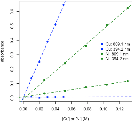
\[ε_\textrm{809.1,Ni}b = 0.837\: \textrm{M}^{–1}\: \textrm{ and }\: ε_\textrm{394.2,Νi}b = 4.870\: \textrm{M}^{–1}\nonumber\]
\[ε_\textrm{809.1,Cu}b = 12.78\: \textrm{M}^{–1}\: \textrm{ and }\: ε_\textrm{394.2,Cu}b = 0.017\: \textrm{M}^{–1}\nonumber\]
-
R functions: plot( ), legend( ), lm( ), abline( )
-
- use R’s solve function to calculate concentrations of copper and nickel in mixture
\[\mathrm{\textit{C}_{Cu} = 0.0182\: M\:\: and\:\: \textit{C}_{Ni} = 0.0506\: M}\nonumber\]
2×2 matrix of εb values
Cu
Ni
809.1 nm
12.77888326
0.8369356
394.2 nm
0.01747073
4.8700205
2×1 matrix of absorbance values
mixture
809.1 nm
0.2789825
394.2 nm
0.2415476
calculate 2×1 matrix of concentrations
[eb] × [conc] = [abs]
mixture
Cu
0.01858748
Ni
0.04953220
-
R functions: matrix( ), colnames( ), rownames( ), solve( )
-
Matrix Notation for Beer’s Law (A = εbC)
two analytes: two samples with absorbance measured at two wavelengths
\[ [A]_\textrm{2 samples × 2 wavelengths} = [C]_\textrm{2 samples × 2 analytes} × [εb]_\textrm{2 analytes × 2 wavelengths} \nonumber\]
one analyte: one sample with absorbance measured at one wavelength
\[ [A]_\textrm{1 sample × 1 wavelength} = [C]_\textrm{1 sample × 1 analyte} × [εb]_\textrm{1 analyte × 1 wavelength} \nonumber\]
overdetermined system: more samples and wavelengths than analytes
\[ [A]_\textrm{8 samples × 5 wavelengths} = [C]_\textrm{8 samples × 2 analytes} × [εb]_\textrm{2 analytes × 5 wavelengths} + [RE]_\textrm{8 samples × 5 wavelengths} \nonumber\]
generalize: n analytes, s samples, and w wavelengths where n ≤ smaller of s or w
\[ [A]_{s × w} = [C]_{s × n} × [εb]_{n × w} + [RE]_{s × w} \nonumber\]
Main Feature
(in 3 Parts w/2 Themes)
How Does PCA Work?
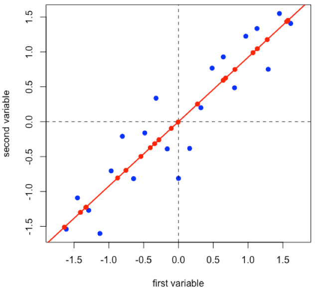
Suppose we have 21 samples and that we measure two properties—first variable and second variable— for each sample giving a matrix of data, [D], that has 21 rows and 2 columns.
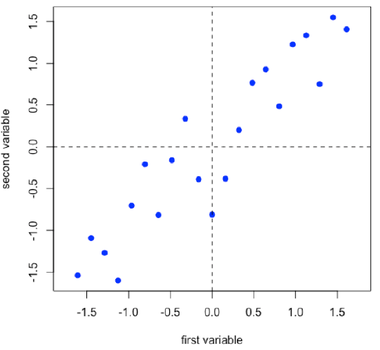
\[ [D]_{21 × 2} \nonumber\]
- R functions: seq( ), rnorm( ), scale( ), plot( ), abline( )
Linear regression provides the line of best fit to the data and explains more of the data’s overall variance than either of the two individual variables; we call this the first principal component.
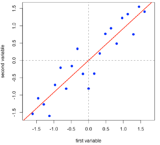
- R functions: lm( ), abline( )
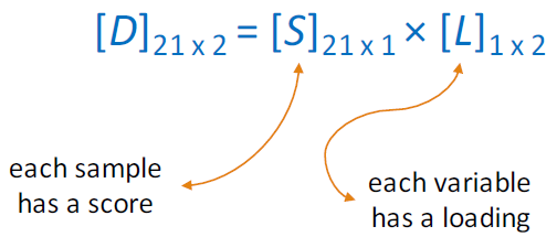
Projecting the data onto the regression line gives the location of the data on the first principal component; these are called scores, (S). The cosines of the angles between the first principal component and each of the original axes are called loadings, (L).
- R functions: points( )
Projecting the original data onto a line that is perpendicular to the first principal component gives the second principal component and adds in a second set of scores and loadings.
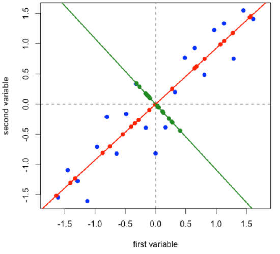
\[ [D]_{21 × 2} = [S]_{21 × 2} × [L]_{2 × 2} \nonumber\]
\[ [A]_{s × w} = [C]_{s × n} × [εb]_{n × w} + [RE]_{s × w} \nonumber\]
- R functions: abline( ), points( )
PCA: Worked Example
\[ [A]_{s × w} = [C]_{s × n} × [εb]_{n × w} + [RE]_{s × w} \nonumber\]
Subset of data consisting of 24 of the 80 samples: stock Cu, stock Co, stock Cr, five Cu/Co binary mixtures, five Cu/Cr binary mixtures, five Co/Cr binary mixtures, six Cu/Co/Cr ternary mixtures.
- choose a subset of the original 635 wavelengths
[1] 380.5 414.9 449.3 483.7 517.9 550.6 583.2 613.3
[9] 642.9 672.7 703.3 735.5 767.8 800.2 832.6 868.7
-
R functions: plot( ), lines( ), abline( ), legend( ), as.numeric( ), colnames( )
-
- perform PCA and determine relative importance of the 16 principal components
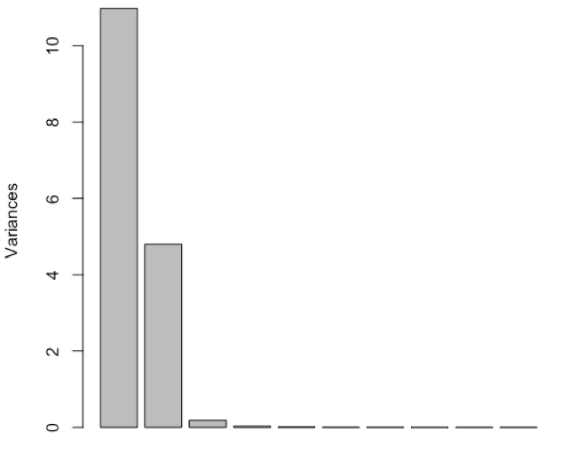
PC1
PC2
PC3
PC4
Standard deviation
3.3134
2.1901
0.42561
0.17585
Proportion of Variance
0.6862
0.2998
0.01132
0.00193
Cumulative Proportion
0.6862
0.9859
0.99725
0.99919
-
R functions: prcomp( ), plot( ), summary( )
-
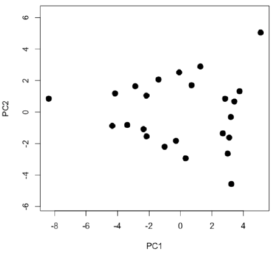
- examine and interpret scores for first two principal components
-
R functions: plot( )

-
R functions: plot( ), factor( ), legend( )
-
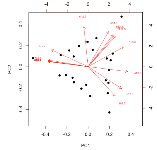
- examine and interpret biplot of loadings and scores for the first two principal components
-
R functions: biplot( )
-
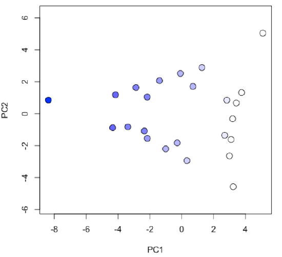
R functions: plot( ), colorRampPalatte( ), as.numeric( ), cut( )
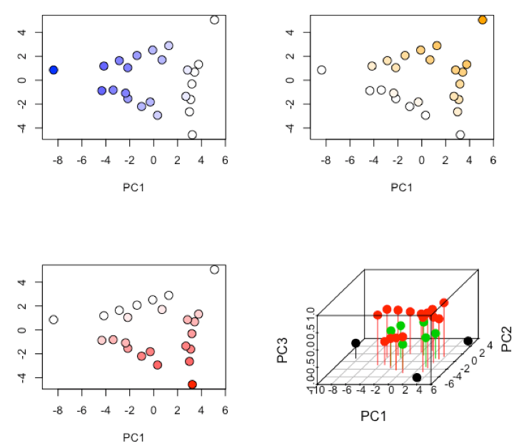
-
R functions: par( ), plot( ), scatterplot3d::scatterplot3d
-
How Does Cluster Analysis Work?
Suppose we have six samples and that we measure two properties—a and b—for each sample and create a scatterplot of the data.
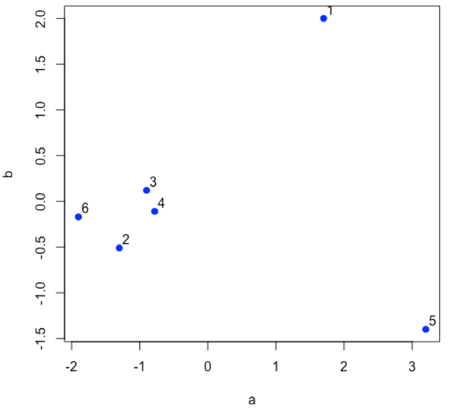
- R functions: plot( )
Find the two points that are closest to each other; this is the first cluster. Find the midpoint between the two points and define it as the position of the first cluster.
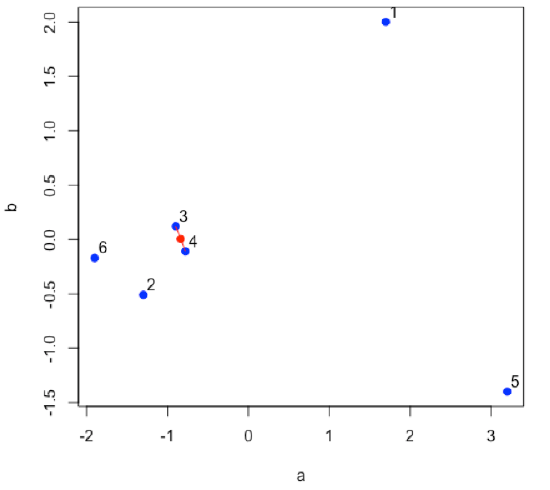
- R functions: plot( ), segments( ), points( )
Find the next two points that are closest to each other; this is the second cluster. Find the midpoint between the two points and define it as the position of the second cluster.
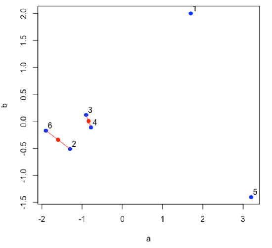
- R functions: plot( ), segments( ), points( )
Continue until all of the original data points are included in a cluster.

- R functions: plot( ), segments( ), points( )
Plot a dendrogram, which shows the connectivity between points and clusters of points in terms of the distance (heights) separating them.
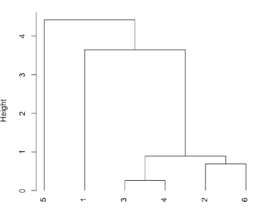
- R functions: dist( ), hclust( ), plot( )
Cluster Analysis: Worked Example
Subset of data consisting of 24 of the 80 samples: stock Cu, stock Co, stock Cr, five Cu/Co binary mixtures, five Cu/Cr binary mixtures, five Co/Cr binary mixtures, six Cu/Co/Cr ternary mixtures.
- calculate the distance between the individual data points using one of the available methods
1
2
3
4
5
2
1.53328104
3
1.73128979
0.96493008
4
1.48359716
0.24997370
0.77766228
5
1.49208058
0.32863786
0.68852029
0.09664215
6
1.49457333
0.42903074
0.57495499
0.21089686
0.11755129
-
R functions: dist( )
-
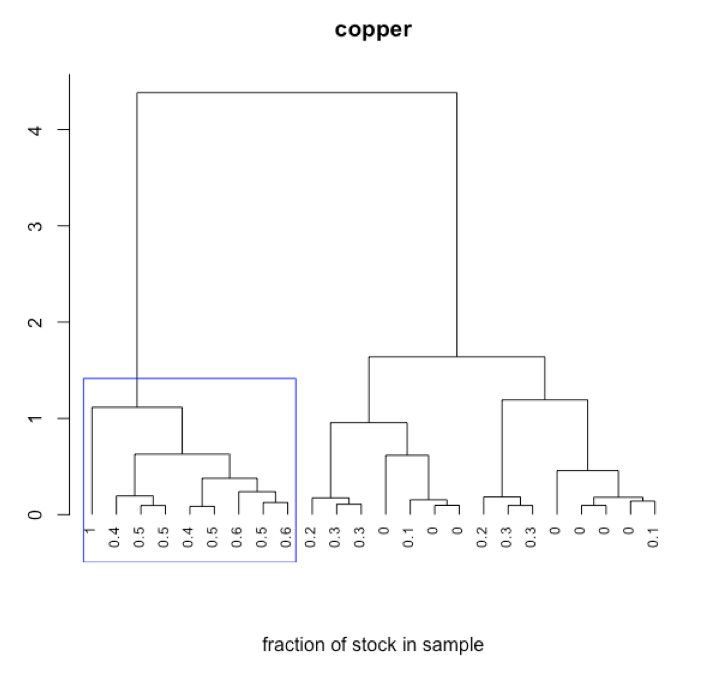
- identify clusters and calculate and plot the heights between them using one of the available methods

-
R functions: hclust( ), plot( )
-
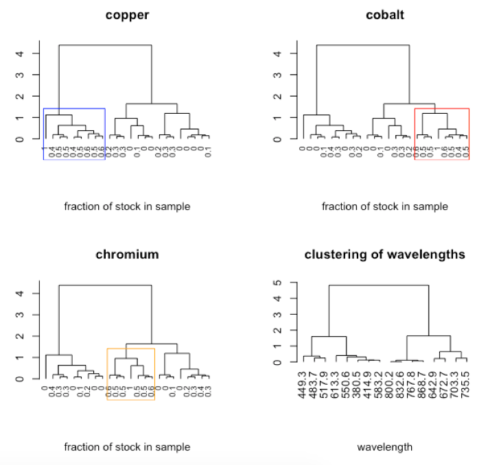
- interpret dendrogram
-
R functions: plot( ), rect.hclust( )
-
R functions: par( ), plot( ), rect.hclust( ), t( )
-
How Does MLR Work?
\[ [A]_{s × w} = [C]_{s × n} × [εb]_{n × w} \nonumber\]
Suppose we measure the absorbance at W wavelengths for S individual standard solutions with known concentrations for each of the N analytes. We can use these to determine a matrix of εb values for each analyte at each wavelength.
\[ [C]^\textrm{T}_{n × s} × [A]_{s × w} = [C]^\textrm{T}_{n × s} × [C]_{s × n} × [εb]_{n × w} \nonumber\]
\[ ([C]^\textrm{T}_{n × s} × [C]_{s × n})^{–1} ×[C]^\textrm{T}_{n × c}×[A]_{s × w} = ([C]^\textrm{T}_{n × n}×[C]_{s × n})^{–1} ×[C]^\textrm{T}_{n × s}×[C]_{s × n}×[εb]_{n × w} \nonumber\]
\[ ([C]^\textrm{T}_{s × n} × [C]_{s × n})^{–1} ×[C]^\textrm{T}_{s × n}×[A]_{s × w} = [εb]_{n × w} \nonumber\]
Having found the εb matrix, we can use it to calculate the concentrations for each of the N analytes in S samples given the absorbance for each sample at each wavelength.
\[ [A]_{s×w}×[εb]^\textrm{T}_{w×n} = [C]_{s×n}×[εb]_{n×w}×[εb]^\textrm{T}_{w×n} \nonumber\]
\[ [A]_{s×w}×[εb]^\textrm{T}_{w×n}× ([εb]_{n×w}×[εb]^\textrm{T}_{w×n})^{–1} = [C]_{s×n}×[εb]_{n×w}×[εb]^\textrm{T}_{w×n}× ([εb]_{n×w}×[εb]^\textrm{T}_{w×n})^{–1} \nonumber\]
\[ [A]_{s×w}×[εb]^\textrm{T}_{w×n}× ([εb]_{n×w}×[εb]^\textrm{T}_{w×n})^{–1} = [C]_{s×n} \nonumber\]
MLR: Worked Example
Standards are subset of data consisting of 15 of the 80 samples: five each prepared from stock Cu, stock Co, and stock Cr. Samples are subset of data consisting of 21 of the 80 samples: five Cu/Co binary mixtures, five Cu/Cr binary mixtures, five Co/Cr binary mixtures, six Cu/Co/Cr ternary mixtures.
- use absorbance values for a set of standards to calculate the εb values
380.5
414.9
449.3
483.7
517.9
550.6
583.2
613.3
concCu
0.5484511
0.1086153
0.1340763
0.1556545
0.1947192
0.3612272
0.6875421
1.3197158
concCo
0.7117778
0.7918523
2.5371205
4.0549583
4.5779242
2.0489508
0.5975168
0.3914665
concCr
13.2668054
15.1576056
6.9958232
4.0685312
6.7662738
12.0692592
13.6134665
9.8289364
-
R functions: findeb( )* * script written for this purpose
-
- use absorbance values for the samples and the calculated εb values to give the predicted concentrations of the analytes
predicted concentrations of analytes
concCu
concCo
concCr
[1,]
-0.00024
0.05991
0.00696
[2,]
-0.00037
0.04939
0.01050
[3,]
0.00036
0.03926
0.01488
[4,]
0.00075
0.03088
0.01879
[5,]
-0.00031
0.01947
0.02227
[6,]
0.01040
0.06076
0.00079
-
R functions: findconc( )* * script written for this purpose
-
- compare predicted and actual concentrations
actual concentrations of analytes
concCu
concCo
concCr
[1,]
0.000
0.06
0.00750
[2,]
0.000
0.05
0.01125
[3,]
0.000
0.04
0.01500
[4,]
0.000
0.03
0.01875
[5,]
0.000
0.02
0.02250
[6,]
0.010
0.06
0.00000
-
R functions: as.matrix( ), data.frame( )
-
- report mean errors, standard deviations for errors, confidence intervals for errors, and identify maximum error for each analyte
mean errors
concCu
concCo
concCr
-0.000304
-0.000199
-0.000315
standard deviations for errors
concCu
concCo
concCr
0.001102
0.000857
0.000662
confidence intervals for errors
concCu
concCo
concCr
±0.002298
±0.001787
±0.001381
maximum error
Cu: 0.00219 (0.02719 vs. 0.0250)
Co: 0.00176 (0.05176 vs. 0.0500)
Cr: 0.00173 (0.00173 vs. 0)*
* exceeds 95% confidence interval
-
R functions: as.matrix( ), data.frame( ), apply( ), which.max( ), abs( ), round( )
-
Contributors and Attributions
- David Harvey, Depauw University (harvey@depauw.edu)
- Sourced from the Analytical Sciences Digital Library
Acknowledgments
- students in Chem 351
- Brian Saulnier (DePauw Chemistry major, class of 2018)
- DePauw University’s Faculty Development Committee
- stackoverflow