10.1: Emission Spectroscopy Based on Flame and Plasma Sources

What is Emission?

An analyte in an excited state possesses an energy, E₂, that is greater than its energy when it is in a lower energy state, E₁. When the analyte returns to its lower energy state—a process we call relaxation—the excess energy, \(\Delta E\), is

\[\Delta E=E_{2}-E_{1} \nonumber \]

There are several ways in which an atom may end up in an excited state, including thermal energy, which is the focus of this chapter. The amount of time an atom, A, spends in its excited state—what we call the excited state's lifetime—is short, typically \(10^{-5}\) to \(10^{-9}\) s for an electronic excited state. Relaxation of the atom's excited state, A*, occurs through several mechanisms, including collisions with other species in the sample and the emission of photons. In the first process, which we call nonradiative relaxation, the excess energy is released as heat.

\[A^{*} \longrightarrow A+\text { heat } \nonumber \]

In the second mechanism, the excess energy is released as a photon of electromagnetic radiation.

\[A^{*} \longrightarrow A+h \nu \nonumber \]

The release of a photon following thermal excitation is called emission. The focus of this chapter is on the emission of ultraviolet and visible radiation following the thermal excitation of atoms. Atomic emission spectroscopy has a long history. Qualitative applications based on the color of flames were used in the smelting of ores as early as 1550 and were more fully developed around 1830 with the observation of atomic spectra generated by flame emission and spark emission [Dawson, J. B. J. Anal. At. Spectrosc. 1991, 6, 93–98]. Quantitative applications based on the atomic emission from electric sparks were developed by Lockyer in the early 1870 and quantitative applications based on flame emission were pioneered by Lundegardh in 1930. Atomic emission based on emission from a plasma was introduced in 1964.

Atomic Emission Spectra

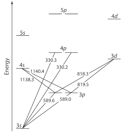
Atomic emission occurs when a valence electron in a higher energy atomic orbital returns to a lower energy atomic orbital. Figure \(\PageIndex{1}\) shows a portion of the energy level diagram for sodium, which consists of a series of discrete lines at wavelengths that correspond to the difference in energy between two atomic orbitals.

FFigure \(\PageIndex{1}\). Valence shell energy level diagram for sodium. The wavelengths corresponding to several transitions are shown.

The intensity of an atomic emission line, I_e, is proportional to the number of atoms, \(N^*\), that populate the excited state

\[I_{e}=k N^* \label{10.1} \]

where k is a constant that accounts for the efficiency of the transition. If a system of atoms is in thermal equilibrium, the population of excited state i is related to the total concentration of atoms, N, by the Boltzmann distribution. For many elements at temperatures of less than 5000 K the Boltzmann distribution is approximated as

\[N^* = N\left(\frac{g_{i}}{g_{0}}\right) e^{-E_i / k T} \label{10.2} \]

where g_i and g₀ are statistical factors that account for the number of equivalent energy levels for the excited state and the ground state, E_i is the energy of the excited state relative to the ground state, E₀, k is Boltzmann’s constant (\(1.3807 \times 10^{-23}\) J/K), and T is the temperature in Kelvin. From Equation \ref{10.2} we expect that excited states with lower energies have larger populations and more intense emission lines. We also expect emission intensity to increase with temperature. The emission spectrum for sodium is shown in Figure \(\PageIndex{2}\)

Figure \(\PageIndex{2}\): Visible emission spectrum for sodium. The inset shows a close up of the emission lines at 589.0 and 589.6 nm that appear in the energy level diagram in Figure \(\PageIndex{1}\).

An atomic emission spectrometer is similar in design to the instrumentation for atomic absorption. In fact, it is easy to adapt most flame atomic absorption spectrometers for atomic emission by turning off the hollow cathode lamp and monitoring the difference between the emission intensity when aspirating the sample and when aspirating a blank. Many atomic emission spectrometers, however, are dedicated instruments designed to take advantage of features unique to atomic emission, including the use of plasmas, arcs, sparks, and lasers as atomization and excitation sources, and an enhanced capability for multielemental analysis.

Flames as a Source

Atomization and excitation in flame atomic emission is accomplished with the same nebulization and spray chamber assembly used in atomic absorption (see Chapter 9). The burner head consists of a single or multiple slots, or a Meker-style burner. Older atomic emission instruments often used a total consumption burner in which the sample is drawn through a capillary tube and injected directly into the flame.

A Meker burner is similar to the more common Bunsen burner found in most laboratories; it is designed to allow for higher temperatures and for a larger diameter flame.

The Inductively Coupled Plasma Source

A plasma is a hot, partially ionized gas that contains an abundant concentration of cations and electrons. The plasma used in atomic emission is formed by ionizing a flowing stream of argon gas, producing argon ions and electrons. A plasma’s high temperature results from resistive heating as the electrons and argon ions move through the gas. Because a plasma operates at a much higher temperature than a flame, it provides for a better atomization efficiency and a higher population of excited states.

A schematic diagram of the inductively coupled plasma source (ICP) is shown in Figure \(\PageIndex{3}\). The ICP torch consists of three concentric quartz tubes, surrounded at the top by a radio-frequency induction coil. The sample is mixed with a stream of Ar using a nebulizer, and is carried to the plasma through the torch’s central capillary tube. Plasma formation is initiated by a spark from a Tesla coil. An alternating radio-frequency current in the induction coil creates a fluctuating magnetic field that induces the argon ions and the electrons to move in a circular path. The resulting collisions with the abundant unionized gas give rise to resistive heating, providing temperatures as high as 10000 K at the base of the plasma, and between 6000 and 8000 K at a height of 15–20 mm above the coil, where emission usually is measured. At these high temperatures the outer quartz tube must be thermally isolated from the plasma. This is accomplished by the tangential flow of argon shown in the schematic diagram. Samples are brought into the ICP using the same basic types of nebulization described in Chapter 8 for flame atomic absorption spectroscopy.

Figure \(\PageIndex{3}\). Schematic diagram of an inductively coupled plasma torch for atomic emission.

The Direct Current Plasma Source

An alternative to the inductively coupled plasma source is the direct current (dc) plasma jet, one example of which is illustrated in Figure \(\PageIndex{4}\). The argon plasma (shown here in blue) forms between two graphite anodes and a tungsten cathode. The sample is aspirated into the plasma's excitation region where it undergoes atomization, excitation, and emission at temperatures of 5000 K.

Figure \(\PageIndex{4}\): Illustration showing a schematic diagram of a direct current plasma source of atomic emission.

Flame and Plasma Spectrometers

One advantage of atomic emission over atomic absorption is the ease of analyzing samples for multiple analytes. This additional capability arises because atomic emission, unlike atomic absorption, does not need an analyte-specific source of radiation. The two most common types of spectrometers are sequential and multichannel. In a sequential spectrometer the instrument has a single detector and uses the monochromator to move from one emission line to the next. A multichannel spectrometer uses the monochromator to disperse the emission across a field of detectors, each of which measures the emission intensity at a different wavelength.

Sequential Instruments

A sequential instrument uses a programmable scanning monochromator, such as those described in Chapter 7, to rapidly move the monochromator's grating over wavelength regions that are not of interest, and then pauses and scans slowly over the emission lines of the analytes. Sampling rates of 300 determinations per hour are possible with this configuration. Another option, which is less common, is to move the exit slit and the detector across the monochromator's focal plane, pausing and recording the emission at the desired wavelengths.

Multichannel Instruments

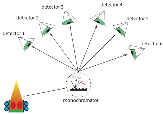
Another approach to a multielemental analysis is to use a multichannel instrument that allows us to monitor simultaneously many analytes. A simple design for a multichannel spectrometer, shown in Figure \(\PageIndex{5}\), couples a monochromator with multiple detectors that are positioned in a semicircular array around the monochromator at positions that correspond to the wavelengths for the analytes. A sample throughput of 3000 determinations per hour are possible using a multichannel ICP.

Figure \(\PageIndex{5}\). Schematic diagram of a multichannel atomic emission spectrometer for the simultaneous analysis of several elements. Instruments may contain as many as 48–60 detectors.

Another option for a multichannel instrument takes advantage of the charge-injection device, or CID, as a detector (see Chapter 7 for discussion of the charge-coupled device, another type of charge-transfer device used as a detector). Light from the plasma source is dispersed across the CID in two dimensions. The surface of the CID has in excess of 90000 detecting elements, or pixels, that allows for a resolution between detecting elements on the order of 0.04 nm. Light from the atomic emission source is distributed across the detector's surface by a diffraction grating such that each element of interest is detected using its own set of pixels, called a read window. Figure \(\PageIndex{6}\) shows that individual read windows consist of a set of detecting elements, nine of which collect photons from the spectral line and 30 of which provide a measurement of the source's background.

Figure \(\PageIndex{6}\): Illustration showing a charge-injection detector. The read window consists of nine central elements that measure the analyte's emission intensity (shown here using blue shading) and 30 of which measure the background emission from the plasma source.

Application of Flame and Plasma Sources

Atomic emission is used widely for the analysis of trace metals in a variety of sample matrices. The development of a quantitative atomic emission method requires several considerations, including choosing a source for atomization and excitation, selecting a wavelength and slit width, preparing the sample for analysis, minimizing spectral and chemical interferences, and selecting a method of standardization.

Choice of Atomization and Excitation Source

Except for the alkali metals, detection limits when using an ICP are significantly better than those obtained with flame emission (Table \(\PageIndex{1}\)). Plasmas also are subject to fewer spectral and chemical interferences. For these reasons a plasma emission source is usually the better choice.

Table \(\PageIndex{1}\). Detection Limits for Atomic Emission

element	detection limit (µg/mL): flame emission	detection limit (µg/mL): ICP
Ag	2	0.2
Al	3	0.2
As	2000	2
Ca	0.1	0.0001
Cd	300	0.07
Co	5	0.1
Cr	1	0.08
Fe	10	0.09
Hg	150	1
K	0.01	30
Li	0.001	0.02
Mg	1	0.02
Mn	1	0.01
Na	0.01	0.1
Ni	10	0.2
Pb	0.2	1
Pt	2000	0.9
Sn	100	3
Zn	1000	0.1
Source: Parsons, M. L.; Major, S.; Forster, A. R.; App. Spectrosc. 1983, 37, 411–418.

Selecting the Wavelength and Slit Width

The choice of wavelength is dictated by the need for sensitivity and the need to avoid interferences from the emission lines of other constituents in the sample. Because an analyte’s atomic emission spectrum has an abundance of emission lines—particularly when using a high temperature plasma source—it is inevitable that there will be some overlap between emission lines. For example, an analysis for Ni using the atomic emission line at 349.30 nm is complicated by the atomic emission line for Fe at 349.06 nm.

A narrower slit width provides better resolution, but at the cost of less radiation reaching the detector. The easiest approach to selecting a wavelength is to record the sample’s emission spectrum and look for an emission line that provides an intense signal and is resolved from other emission lines.

Preparing the Sample

Flame and plasma sources are best suited for samples in solution and in liquid form. Although a solid sample can be analyzed by directly inserting it into the flame or plasma, they usually are first brought into solution by digestion or extraction.

Minimizing Spectral Interferences

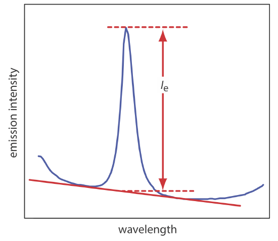
The most important spectral interference is broad, background emission from the flame or plasma and emission bands from molecular species. This background emission is particularly severe for flames because the temperature is insufficient to break down refractory compounds, such as oxides and hydroxides. Background corrections for flame emission are made by scanning over the emission line and drawing a baseline (Figure \(\PageIndex{7}\)). Because a plasma’s temperature is much higher, a background interference due to molecular emission is less of a problem. Although emission from the plasma’s core is strong, it is insignificant at a height of 10–30 mm above the core where measurements normally are made.

Figure \(\PageIndex{7}\). Method for correcting an analyte’s emission for the flame’s background emission.

Minimizing Chemical Interferences

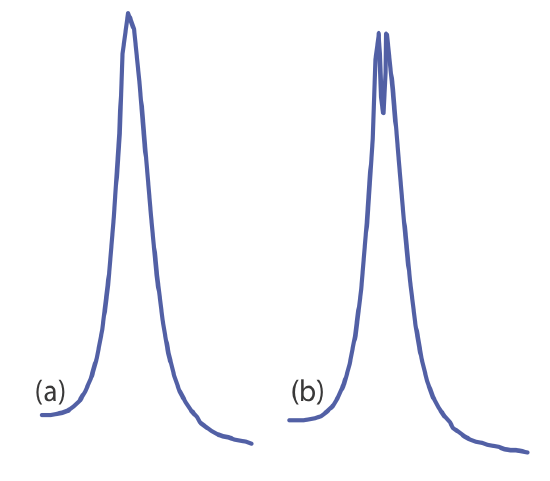
Flame emission is subject to the same types of chemical interferences as atomic absorption; they are minimized using the same methods: by adjusting the flame’s composition and by adding protecting agents, releasing agents, or ionization suppressors. An additional chemical interference results from self-absorption. Because the flame’s temperature is greatest at its center, the concentration of analyte atoms in an excited state is greater at the flame’s center than at its outer edges. If an excited state atom in the flame’s center emits a photon, then a ground state atom in the cooler, outer regions of the flame may absorb the photon, which decreases the emission intensity. For higher concentrations of analyte self-absorption may invert the center of the emission band (Figure \(\PageIndex{8}\)).

Figure \(\PageIndex{8}\). Atomic emission lines for (a) a low concentration of analyte, and (b) a high concentration of analyte showing the effect of self-absorption.

Chemical interferences when using a plasma source generally are not significant because the plasma’s higher temperature limits the formation of nonvolatile species. For example, \(\text{PO}_4^{3-}\) is a significant interferent when analyzing samples for Ca²⁺ by flame emission, but has a negligible effect when using a plasma source. In addition, the high concentration of electrons from the ionization of argon minimizes ionization interferences.

Standardizing the Method

From Equation \ref{10.1} we know that emission intensity is proportional to the population of the analyte’s excited state, \(N^*\). If the flame or plasma is in thermal equilibrium, then the excited state population is proportional to the analyte’s total population, N, through the Boltzmann distribution (Equation \ref{10.2}).

A calibration curve for flame emission usually is linear over two to three orders of magnitude, with ionization limiting linearity when the analyte’s concentrations is small and self-absorption limiting linearity at higher concentrations of analyte. When using a plasma, which suffers from fewer chemical interferences, the calibration curve often is linear over four to five orders of magnitude and is not affected significantly by changes in the matrix of the standards.

Emission intensity is affected significantly by many parameters, including the temperature of the excitation source and the efficiency of atomization. An increase in temperature of 10 K, for example, produces a 4% increase in the fraction of Na atoms in the 3p excited state, an uncertainty in the signal that may limit the use of external standards. The method of internal standards is used when the variations in source parameters are difficult to control. To compensate for changes in the temperature of the excitation source, the internal standard is selected so that its emission line is close to the analyte’s emission line. In addition, the internal standard should be subject to the same chemical interferences to compensate for changes in atomization efficiency. To accurately correct for these errors the analyte and internal standard emission lines are monitored simultaneously.