
What is Chemometrics and Why Study it?
- Page ID
- 218837

\( \newcommand{\vecs}[1]{\overset { \scriptstyle \rightharpoonup} {\mathbf{#1}} } \)
\( \newcommand{\vecd}[1]{\overset{-\!-\!\rightharpoonup}{\vphantom{a}\smash {#1}}} \)
\( \newcommand{\dsum}{\displaystyle\sum\limits} \)
\( \newcommand{\dint}{\displaystyle\int\limits} \)
\( \newcommand{\dlim}{\displaystyle\lim\limits} \)
\( \newcommand{\id}{\mathrm{id}}\) \( \newcommand{\Span}{\mathrm{span}}\)
( \newcommand{\kernel}{\mathrm{null}\,}\) \( \newcommand{\range}{\mathrm{range}\,}\)
\( \newcommand{\RealPart}{\mathrm{Re}}\) \( \newcommand{\ImaginaryPart}{\mathrm{Im}}\)
\( \newcommand{\Argument}{\mathrm{Arg}}\) \( \newcommand{\norm}[1]{\| #1 \|}\)
\( \newcommand{\inner}[2]{\langle #1, #2 \rangle}\)
\( \newcommand{\Span}{\mathrm{span}}\)
\( \newcommand{\id}{\mathrm{id}}\)
\( \newcommand{\Span}{\mathrm{span}}\)
\( \newcommand{\kernel}{\mathrm{null}\,}\)
\( \newcommand{\range}{\mathrm{range}\,}\)
\( \newcommand{\RealPart}{\mathrm{Re}}\)
\( \newcommand{\ImaginaryPart}{\mathrm{Im}}\)
\( \newcommand{\Argument}{\mathrm{Arg}}\)
\( \newcommand{\norm}[1]{\| #1 \|}\)
\( \newcommand{\inner}[2]{\langle #1, #2 \rangle}\)
\( \newcommand{\Span}{\mathrm{span}}\) \( \newcommand{\AA}{\unicode[.8,0]{x212B}}\)
\( \newcommand{\vectorA}[1]{\vec{#1}} % arrow\)
\( \newcommand{\vectorAt}[1]{\vec{\text{#1}}} % arrow\)
\( \newcommand{\vectorB}[1]{\overset { \scriptstyle \rightharpoonup} {\mathbf{#1}} } \)
\( \newcommand{\vectorC}[1]{\textbf{#1}} \)
\( \newcommand{\vectorD}[1]{\overrightarrow{#1}} \)
\( \newcommand{\vectorDt}[1]{\overrightarrow{\text{#1}}} \)
\( \newcommand{\vectE}[1]{\overset{-\!-\!\rightharpoonup}{\vphantom{a}\smash{\mathbf {#1}}}} \)
\( \newcommand{\vecs}[1]{\overset { \scriptstyle \rightharpoonup} {\mathbf{#1}} } \)
\(\newcommand{\longvect}{\overrightarrow}\)
\( \newcommand{\vecd}[1]{\overset{-\!-\!\rightharpoonup}{\vphantom{a}\smash {#1}}} \)
\(\newcommand{\avec}{\mathbf a}\) \(\newcommand{\bvec}{\mathbf b}\) \(\newcommand{\cvec}{\mathbf c}\) \(\newcommand{\dvec}{\mathbf d}\) \(\newcommand{\dtil}{\widetilde{\mathbf d}}\) \(\newcommand{\evec}{\mathbf e}\) \(\newcommand{\fvec}{\mathbf f}\) \(\newcommand{\nvec}{\mathbf n}\) \(\newcommand{\pvec}{\mathbf p}\) \(\newcommand{\qvec}{\mathbf q}\) \(\newcommand{\svec}{\mathbf s}\) \(\newcommand{\tvec}{\mathbf t}\) \(\newcommand{\uvec}{\mathbf u}\) \(\newcommand{\vvec}{\mathbf v}\) \(\newcommand{\wvec}{\mathbf w}\) \(\newcommand{\xvec}{\mathbf x}\) \(\newcommand{\yvec}{\mathbf y}\) \(\newcommand{\zvec}{\mathbf z}\) \(\newcommand{\rvec}{\mathbf r}\) \(\newcommand{\mvec}{\mathbf m}\) \(\newcommand{\zerovec}{\mathbf 0}\) \(\newcommand{\onevec}{\mathbf 1}\) \(\newcommand{\real}{\mathbb R}\) \(\newcommand{\twovec}[2]{\left[\begin{array}{r}#1 \\ #2 \end{array}\right]}\) \(\newcommand{\ctwovec}[2]{\left[\begin{array}{c}#1 \\ #2 \end{array}\right]}\) \(\newcommand{\threevec}[3]{\left[\begin{array}{r}#1 \\ #2 \\ #3 \end{array}\right]}\) \(\newcommand{\cthreevec}[3]{\left[\begin{array}{c}#1 \\ #2 \\ #3 \end{array}\right]}\) \(\newcommand{\fourvec}[4]{\left[\begin{array}{r}#1 \\ #2 \\ #3 \\ #4 \end{array}\right]}\) \(\newcommand{\cfourvec}[4]{\left[\begin{array}{c}#1 \\ #2 \\ #3 \\ #4 \end{array}\right]}\) \(\newcommand{\fivevec}[5]{\left[\begin{array}{r}#1 \\ #2 \\ #3 \\ #4 \\ #5 \\ \end{array}\right]}\) \(\newcommand{\cfivevec}[5]{\left[\begin{array}{c}#1 \\ #2 \\ #3 \\ #4 \\ #5 \\ \end{array}\right]}\) \(\newcommand{\mattwo}[4]{\left[\begin{array}{rr}#1 \amp #2 \\ #3 \amp #4 \\ \end{array}\right]}\) \(\newcommand{\laspan}[1]{\text{Span}\{#1\}}\) \(\newcommand{\bcal}{\cal B}\) \(\newcommand{\ccal}{\cal C}\) \(\newcommand{\scal}{\cal S}\) \(\newcommand{\wcal}{\cal W}\) \(\newcommand{\ecal}{\cal E}\) \(\newcommand{\coords}[2]{\left\{#1\right\}_{#2}}\) \(\newcommand{\gray}[1]{\color{gray}{#1}}\) \(\newcommand{\lgray}[1]{\color{lightgray}{#1}}\) \(\newcommand{\rank}{\operatorname{rank}}\) \(\newcommand{\row}{\text{Row}}\) \(\newcommand{\col}{\text{Col}}\) \(\renewcommand{\row}{\text{Row}}\) \(\newcommand{\nul}{\text{Nul}}\) \(\newcommand{\var}{\text{Var}}\) \(\newcommand{\corr}{\text{corr}}\) \(\newcommand{\len}[1]{\left|#1\right|}\) \(\newcommand{\bbar}{\overline{\bvec}}\) \(\newcommand{\bhat}{\widehat{\bvec}}\) \(\newcommand{\bperp}{\bvec^\perp}\) \(\newcommand{\xhat}{\widehat{\xvec}}\) \(\newcommand{\vhat}{\widehat{\vvec}}\) \(\newcommand{\uhat}{\widehat{\uvec}}\) \(\newcommand{\what}{\widehat{\wvec}}\) \(\newcommand{\Sighat}{\widehat{\Sigma}}\) \(\newcommand{\lt}{<}\) \(\newcommand{\gt}{>}\) \(\newcommand{\amp}{&}\) \(\definecolor{fillinmathshade}{gray}{0.9}\)What is Chemometrics?
The definition of chemometrics is is evident in its name, where chemo– means chemical and –metrics means measurement; thus, chemometrics is the study of chemical (and biochemical) measurements and is a branch of analytical chemistry. Examples of chemometric applications include
- ensuring that the data we collect is appropriate for our purposes
- enhancing the quality of an analytical signal by finding ways to minimize the contribution of noise
- reporting on an experiment in a way that estimates the uncertainty in its results and our confidence in those results
- building useful models that predict the outcomes of future experiments
- extracting from chemical data, hidden, but analytically useful information by finding underlying patterns in the data
These topics, and others, are the focus of this textbook.
Why Study Chemometrics?
Why chemometrics is important becomes clear when we consider a simple analytical problem: How do we determine the concentration of copper in a sample, and how and why has the analytical method used for this analysis changed over time.
Prior to the 1950s, gravimetry and titrimetry were the most common analytical methods for determining the concentration of copper in a variety of samples. Both of these methods rely on simple stoichiometric relationships. In a gravimetric analysis, for example, we bring copper into solution as Cu2+(aq), precipitate it as Cu(OH)2(s)
\[\text{Cu}^{2+}(aq) + 2 \text{OH}^{–}(aq) \rightarrow \text{Cu(OH)}_{2}(s) \nonumber\]
and isolate it as CuO(s) after heating it to a high temperature.
\[\text{Cu(OH)}_{2}(s) \rightarrow \text{CuO}(s) + \text{H}_{2}\text{O}(l) \nonumber\]
We then use the mass of CuO(s) to determine the amount of copper in the original sample by accounting for the simple stoichiometric relationship between Cu and CuO where each mole of Cu yields one mole of CuO.
You can read more about gravimetry in Chapter 8 of the textbook Analytical Chemistry 2.1.
In a titrimetric analysis, we bring copper into solution as Cu2+(aq) and slowly add a solution of ethlyenediaminetetracetic acid, EDTA, until the moles of EDTA added is equal to the moles of Cu2+ in the original sample.
\[\text{Cu}^{2+}(aq) + \text{EDTA}(aq) \rightarrow \text{Cu(EDTA)}^{2+}(aq) \nonumber\]
If we know the concentration of our EDTA solution, then it is easy to determine the amount of Cu2+ in the original sample using the simple stoichiometric relationship between Cu2+ and EDTA. For both of these analyses, a chemometric treatment of the data consists of little more than reporting an average, a standard deviation, and a confidence interval.
You can read more about titrimetry in Chapter 9 of the textbook Analytical Chemistry 2.1.
Gravimetry and titrimetry are useful analytical methods when copper is a major (> 1% w/w) analyte or a minor analyte (0.01% w/w – 1% w/w) analyte, but less useful if it is a trace analyte (10−7% w/w – 0.01% w/w). Neither method affords a rapid analysis, which makes them less useful if we need to analyze multiple analytes in a large number of samples.
For more information about the scale of operations for analytical chemistry, including the relative concentrations of analytes in samples, see Chapter 3.4 of the textbook Analytical Chemistry 2.1.
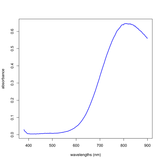
Beginning in the 1950s, instrumental methods of analysis emerged in which an analytical signal is related to the analyte’s concentration, not through the stoichiometry of one or more chemical reactions, but through a theoretical relationship in which at least one variable is not known to us. For example, a solution of Cu2+(aq) is light blue in color because it absorbs light over a broad range of wavelengths between about 600–900 nm, as we see in Figure \(\PageIndex{1}\).
The relationship between a solution’s absorbance, \(A_{\lambda}\), at a specific wavelength, \(\lambda\), and a given concentration, C, of Cu2+(aq) is given by Beer’s law
\[A_{\lambda} = \epsilon_{\lambda} b C \nonumber\]
where \(\epsilon_{\lambda}\) is the analyte’s molar absorptivity at the selected wavelength, \(\lambda\), and b is the distance light travels through the sample. Of these variables—\(A_{\lambda}\), \(\epsilon_{\lambda}\), b, and C—the value of \(\epsilon_{\lambda}\) is not known to us. Contrast that to gravimetry and titrimetry where we almost always know the exact stoichiometric relationships.
For more information about visible absorption spectroscopy and Beer's Law, see Chapter 10.2 in Analytical Chemistry 2.1.
Although we can measure \(A_{\lambda}\) and b, we cannot calculate C without first determining the value of \(\epsilon_{\lambda}\), which we do using a standard solution for which the concentration of analyte is known, Cstd. If we use a single standard and a single wavelength—which is all early instrumentation allowed—then we have
\[\left[ A_{\lambda, std} \right]_{1\ \times\ 1}\ =\ \left[\epsilon_{\lambda} b \right]_{1\ \times\ 1}\ \times\left[C_{std}\right]_{1\ \times\ 1}\nonumber\]
which we can solve exactly for \(\epsilon_{\lambda}b\). With this value in hand, we can use the sample’s absorbance to calculate the analyte’s concentration in the sample.
Note that we are expressing Beer's Law here using the matrix notation \(\left[ \ \ \right]_{r \times c}\), where r is the number of rows and c is the number of columns in the matrix. In this equation, each matrix holds a single value: an absorbance, a value for \(\epsilon_{\lambda}b\), or a concentration. A matrix with a single value is a scaler. A matrix with a single column or a single row is a vector. The reason for expressing Beer's Law in this way will soon be evident.
If we use c standards instead of one standard, and if we continue to use a single wavelength, then we can write Beer’s law this way
\[\left[\cdots\ A_{\lambda, std}\ \cdots\right]_{1\ \times\ c}\ =\ \left[\epsilon_{\lambda} b\right]_{1\ \times\ 1}\ \times\left[\cdots\ C_{std}\ \cdots\right]_{1\ \times\ c}\ +\ \left[\cdots\ E\ \cdots\right]_{1\ \times\ c} \nonumber\]
where the absorbance values and the concentrations are vectors with dimensions of 1×c (1 wavelength and c standards), where the value of \(\epsilon_{\lambda}b\) is a scalar (a constant), and where we have a vector of residual errors, E, that gives the uncertainties in our measured absorbance values. Having multiple standards provides a new source of information that allows us to consider experimental uncertainty!
Note that the equation \(A_{\lambda ,std} = \epsilon_{\lambda}bC\) is in the form of a straight-line, \(y = \beta_{0}x + \beta_{1}\), for which a standard linear regression analysis returns values for the two constants: the slope, \(\beta_{0}\), which is equivalent to \(\epsilon_{\lambda}b\) and the y-intercept, \(\beta_{1}\), which is equivalent to the residual error.
If we use r wavelengths and c standards, then we can write Beer’s law this way
\[\begin{bmatrix} \cdots & \cdots & \cdots \\ \vdots & A_{\lambda, std} & \vdots \\ \cdots & \cdots & \cdots \end{bmatrix}_{r \times c} = \begin{bmatrix} \vdots \\ \epsilon_{\lambda} b \\ \vdots \end{bmatrix}_{r \times 1} \times [ \cdots C_{std} \cdots]_{1 \times c} + \begin{bmatrix} \cdots & \cdots & \cdots \\ \vdots & E & \vdots \\ \cdots & \cdots & \cdots \end{bmatrix}_{r \times c} \nonumber\]
where the absorbance values and the residual errors are in matrices (with wavelengths in rows and standards in columns), the values for \(\epsilon_{\lambda} b\) at each wavelength are in a vector, and the analyte’s concentration in the standards are in a vector; this is a computationally more difficult form of regression, but, as we will learn in a later chapter, one we can solve.
But we can push this even further! Note that the \(\epsilon_{\lambda}b\) matrix has one column because we are using a single wavelength, and the C matrix has one row because we assumed just one analyte. As long as the number of analytes is less than the smaller of the number of wavelengths or the number of standards, then we can include additional analytes. For example, if we have n analytes, then
\[\begin{bmatrix} \cdots & \cdots & \cdots \\ \vdots & A_{\lambda, std} & \vdots \\ \cdots & \cdots & \cdots \end{bmatrix}_{r \times c} = \begin{bmatrix} \cdots & \cdots & \cdots \\ \vdots & \epsilon_{\lambda} b & \vdots \\ \cdots & \cdots & \cdots \end{bmatrix}_{r \times n} \times \begin{bmatrix} \cdots & \cdots & \cdots \\ \vdots & C_{std} & \vdots \\ \cdots & \cdots & \cdots \end{bmatrix}_{n \times c} + \begin{bmatrix} \cdots & \cdots & \cdots \\ \vdots & E & \vdots \\ \cdots & \cdots & \cdots \end{bmatrix}_{r \times c}\nonumber\]
where each column in the \(\epsilon_{\lambda}b\) matrix holds the \(\epsilon_{\lambda}b\) values for a different analyte at one of our wavelengths, and each row in the C matrix is the concentration of a different analyte in one of our standards; again, we can use linear regression to analyze the data.
Moving from the analysis of a single analyte in a single standard using a single wavelength
\[\left[ A_{\lambda, std} \right]_{1\ \times\ 1}\ =\ \left[\epsilon_{\lambda} b\right]_{1\ \times\ 1}\ \times\left[C_{std}\right]_{1\ \times\ 1} \nonumber\]
to the analysis of multiple analytes using multiple standards and multiple wavelengths
\[\begin{bmatrix} \cdots & \cdots & \cdots \\ \vdots & A_{\lambda, std} & \vdots \\ \cdots & \cdots & \cdots \end{bmatrix}_{r \times c} = \begin{bmatrix} \cdots & \cdots & \cdots \\ \vdots & \epsilon_{\lambda} b & \vdots \\ \cdots & \cdots & \cdots \end{bmatrix}_{r \times n} \times \begin{bmatrix} \cdots & \cdots & \cdots \\ \vdots & C_{std} & \vdots \\ \cdots & \cdots & \cdots \end{bmatrix}_{n \times c} + \begin{bmatrix} \cdots & \cdots & \cdots \\ \vdots & E & \vdots \\ \cdots & \cdots & \cdots \end{bmatrix}_{r \times c} \nonumber\]
required a significant increase in computational power and a significant growth in the capabilities of instrumentation; not surprisingly, new chemometric techniques rely on and are driven by developments in computer science and instrumental analysis! In turn, new chemometric techniques open up new areas of analysis and encourage innovations in computer science and instrumental analysis. This is why chemometrics is an important part of analytical chemistry.