Quantitative Analysis: Nuts and Bolts
- Page ID
- 278755
\( \newcommand{\vecs}[1]{\overset { \scriptstyle \rightharpoonup} {\mathbf{#1}} } \)
\( \newcommand{\vecd}[1]{\overset{-\!-\!\rightharpoonup}{\vphantom{a}\smash {#1}}} \)
\( \newcommand{\dsum}{\displaystyle\sum\limits} \)
\( \newcommand{\dint}{\displaystyle\int\limits} \)
\( \newcommand{\dlim}{\displaystyle\lim\limits} \)
\( \newcommand{\id}{\mathrm{id}}\) \( \newcommand{\Span}{\mathrm{span}}\)
( \newcommand{\kernel}{\mathrm{null}\,}\) \( \newcommand{\range}{\mathrm{range}\,}\)
\( \newcommand{\RealPart}{\mathrm{Re}}\) \( \newcommand{\ImaginaryPart}{\mathrm{Im}}\)
\( \newcommand{\Argument}{\mathrm{Arg}}\) \( \newcommand{\norm}[1]{\| #1 \|}\)
\( \newcommand{\inner}[2]{\langle #1, #2 \rangle}\)
\( \newcommand{\Span}{\mathrm{span}}\)
\( \newcommand{\id}{\mathrm{id}}\)
\( \newcommand{\Span}{\mathrm{span}}\)
\( \newcommand{\kernel}{\mathrm{null}\,}\)
\( \newcommand{\range}{\mathrm{range}\,}\)
\( \newcommand{\RealPart}{\mathrm{Re}}\)
\( \newcommand{\ImaginaryPart}{\mathrm{Im}}\)
\( \newcommand{\Argument}{\mathrm{Arg}}\)
\( \newcommand{\norm}[1]{\| #1 \|}\)
\( \newcommand{\inner}[2]{\langle #1, #2 \rangle}\)
\( \newcommand{\Span}{\mathrm{span}}\) \( \newcommand{\AA}{\unicode[.8,0]{x212B}}\)
\( \newcommand{\vectorA}[1]{\vec{#1}} % arrow\)
\( \newcommand{\vectorAt}[1]{\vec{\text{#1}}} % arrow\)
\( \newcommand{\vectorB}[1]{\overset { \scriptstyle \rightharpoonup} {\mathbf{#1}} } \)
\( \newcommand{\vectorC}[1]{\textbf{#1}} \)
\( \newcommand{\vectorD}[1]{\overrightarrow{#1}} \)
\( \newcommand{\vectorDt}[1]{\overrightarrow{\text{#1}}} \)
\( \newcommand{\vectE}[1]{\overset{-\!-\!\rightharpoonup}{\vphantom{a}\smash{\mathbf {#1}}}} \)
\( \newcommand{\vecs}[1]{\overset { \scriptstyle \rightharpoonup} {\mathbf{#1}} } \)
\(\newcommand{\longvect}{\overrightarrow}\)
\( \newcommand{\vecd}[1]{\overset{-\!-\!\rightharpoonup}{\vphantom{a}\smash {#1}}} \)
\(\newcommand{\avec}{\mathbf a}\) \(\newcommand{\bvec}{\mathbf b}\) \(\newcommand{\cvec}{\mathbf c}\) \(\newcommand{\dvec}{\mathbf d}\) \(\newcommand{\dtil}{\widetilde{\mathbf d}}\) \(\newcommand{\evec}{\mathbf e}\) \(\newcommand{\fvec}{\mathbf f}\) \(\newcommand{\nvec}{\mathbf n}\) \(\newcommand{\pvec}{\mathbf p}\) \(\newcommand{\qvec}{\mathbf q}\) \(\newcommand{\svec}{\mathbf s}\) \(\newcommand{\tvec}{\mathbf t}\) \(\newcommand{\uvec}{\mathbf u}\) \(\newcommand{\vvec}{\mathbf v}\) \(\newcommand{\wvec}{\mathbf w}\) \(\newcommand{\xvec}{\mathbf x}\) \(\newcommand{\yvec}{\mathbf y}\) \(\newcommand{\zvec}{\mathbf z}\) \(\newcommand{\rvec}{\mathbf r}\) \(\newcommand{\mvec}{\mathbf m}\) \(\newcommand{\zerovec}{\mathbf 0}\) \(\newcommand{\onevec}{\mathbf 1}\) \(\newcommand{\real}{\mathbb R}\) \(\newcommand{\twovec}[2]{\left[\begin{array}{r}#1 \\ #2 \end{array}\right]}\) \(\newcommand{\ctwovec}[2]{\left[\begin{array}{c}#1 \\ #2 \end{array}\right]}\) \(\newcommand{\threevec}[3]{\left[\begin{array}{r}#1 \\ #2 \\ #3 \end{array}\right]}\) \(\newcommand{\cthreevec}[3]{\left[\begin{array}{c}#1 \\ #2 \\ #3 \end{array}\right]}\) \(\newcommand{\fourvec}[4]{\left[\begin{array}{r}#1 \\ #2 \\ #3 \\ #4 \end{array}\right]}\) \(\newcommand{\cfourvec}[4]{\left[\begin{array}{c}#1 \\ #2 \\ #3 \\ #4 \end{array}\right]}\) \(\newcommand{\fivevec}[5]{\left[\begin{array}{r}#1 \\ #2 \\ #3 \\ #4 \\ #5 \\ \end{array}\right]}\) \(\newcommand{\cfivevec}[5]{\left[\begin{array}{c}#1 \\ #2 \\ #3 \\ #4 \\ #5 \\ \end{array}\right]}\) \(\newcommand{\mattwo}[4]{\left[\begin{array}{rr}#1 \amp #2 \\ #3 \amp #4 \\ \end{array}\right]}\) \(\newcommand{\laspan}[1]{\text{Span}\{#1\}}\) \(\newcommand{\bcal}{\cal B}\) \(\newcommand{\ccal}{\cal C}\) \(\newcommand{\scal}{\cal S}\) \(\newcommand{\wcal}{\cal W}\) \(\newcommand{\ecal}{\cal E}\) \(\newcommand{\coords}[2]{\left\{#1\right\}_{#2}}\) \(\newcommand{\gray}[1]{\color{gray}{#1}}\) \(\newcommand{\lgray}[1]{\color{lightgray}{#1}}\) \(\newcommand{\rank}{\operatorname{rank}}\) \(\newcommand{\row}{\text{Row}}\) \(\newcommand{\col}{\text{Col}}\) \(\renewcommand{\row}{\text{Row}}\) \(\newcommand{\nul}{\text{Nul}}\) \(\newcommand{\var}{\text{Var}}\) \(\newcommand{\corr}{\text{corr}}\) \(\newcommand{\len}[1]{\left|#1\right|}\) \(\newcommand{\bbar}{\overline{\bvec}}\) \(\newcommand{\bhat}{\widehat{\bvec}}\) \(\newcommand{\bperp}{\bvec^\perp}\) \(\newcommand{\xhat}{\widehat{\xvec}}\) \(\newcommand{\vhat}{\widehat{\vvec}}\) \(\newcommand{\uhat}{\widehat{\uvec}}\) \(\newcommand{\what}{\widehat{\wvec}}\) \(\newcommand{\Sighat}{\widehat{\Sigma}}\) \(\newcommand{\lt}{<}\) \(\newcommand{\gt}{>}\) \(\newcommand{\amp}{&}\) \(\definecolor{fillinmathshade}{gray}{0.9}\)The second unit of this course is built on the foundations of equilibrium. Which will be utilized in titrations, gravimetric, and combustion analysis techniques to quantify an analyte. We must remember that this builds off of the quality controls, statistics, and error minimization from unit one.
Objectives
By the end of this students should be able to:
- Understand the different forms of quantification techniques presented, including multiple titrations, gravimetric analysis, and combustion analysis.
- Perform calculation on all of the aforementioned methods to determine the quantity of an analyte.
- Perform all of the quality control and statistical analysis of the presented methods to determine their absolute and relative quality.
Equilibrium Review
Reading: Chapter 1 (section 5), Exploring Chemical Analysis 5th ed., D. Harris
Memorize the table 8-1 of common strong acids and bases in your book.
Equilibrium Constant
\[aA+bB⇆cC+dD\nonumber\]
\[K= \dfrac{[C]^c [D]^d}{[A]^a [B]^b}\nonumber\]
- How do you define equilibrium?
- What does K tell us?
- What is excluded from the K expression?
STOP
- Consider the reaction above. Assume that the value of the equilibrium constant is very large.
- Which species predominate at equilibrium, reactants or products?
- Which reaction has the larger rate constant, the forward or the reverse?
- Which species predominate at equilibrium, reactants or products?
STOP
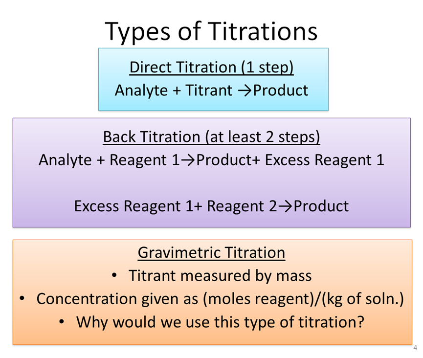
Titration Basics
Reading: Chapter 6 (sections 1-3), Exploring Chemical Analysis 5th ed., D. Harris
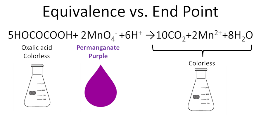
Discuss as a group the following questions
- When is the solution clear?
- When does the solution turn purple?
- What error does this introduce?
- State in your own words the diff b/t equivalence point and end point.
STOP
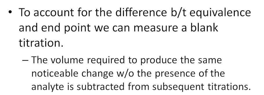
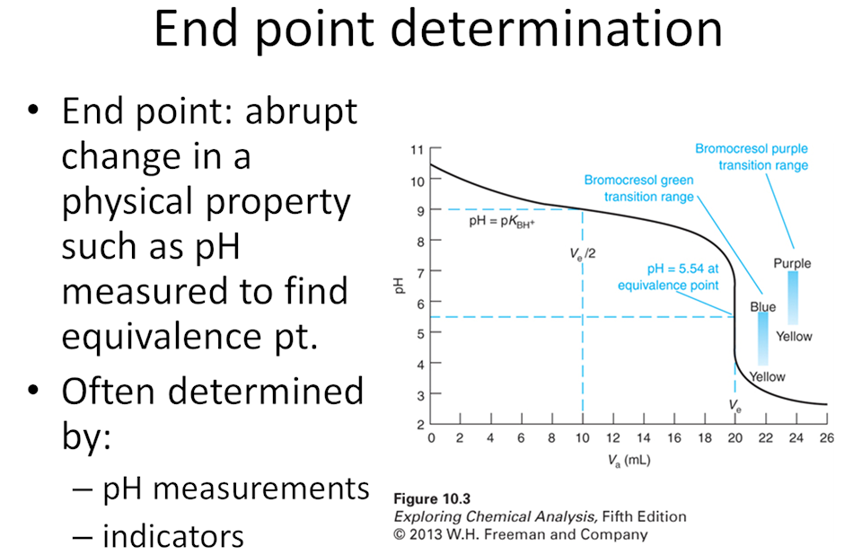
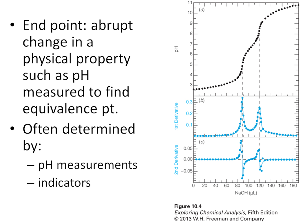
- Think back to when you took general chemistry and you learned how to perform an acid base titration. As a group write out the basic steps to determine the concentration of a weak acid from a titration with a weak base.
STOP
Generic Approach to Quantitative Analysis
*Our known must really be known, how do we get that?
- In the previous unit we learned about primary standards for use in calibration curves, standard addition curves, and internals standards. Can your group think of a way to use a standard to standardize your titrant?
STOP
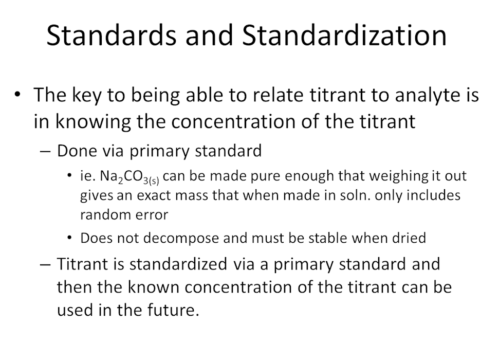
- Standard oxalate was made by dissolving 3.514g of Na2C2O4 (FM 134.00) in 1.000 L of 1 M H2SO4. A 25.00 mL aliquot required 24.44 mL of KMnO4 for titration, and a blank required 0.03 mL of KMnO4. Find the molarity of KMnO4 so it can then be used as a titrant.
\[\ce{5C2O4^2- + 2MnO4- +16H+ → 10CO2 + 2Mn^2+ + 8H2O}\nonumber\]
STOP
- A 20.00 mL aliquot of unknown oxalic acid solution required 17.81 mL of 0.01131 M KMnO4 solution to reach the purple end point. A blank titration of 10 mL of similar solution containing no oxalic acid required 0.02 mL to exhibit detectable color. What is the concentration of the oxalic acid unknown?
STOP
Solubility Product and Common Ion Effect
Reading: Chapter 6 (sections 4-6), Exploring Chemical Analysis 5th ed., D. Harris
- As a group decided how would you explain solubility product (Ksp).
STOP
- What is the concentration of Pb2+ in a saturated PbI2 solution if you know the Ksp=7.9×10‑9?
- What is the concentration of I- in the same PbI2 solution?
STOP
- Which way would the previous reaction for the solubility of PbI2 go if you tried to dissolve PbI2 in a solution NaI? Why?
STOP
- Instead of just dissolving PbI2(s) in H2O let's dissolve it in the presence of 0.0300 M NaI(s) which dissociates completely. What is the concentration of Pb2+ in solution? *note sometimes we need to make approximations to neglect small contributors to the value so we can solve eqn.
STOP
- If I add Ag+ to a mixture of I- and Cl- which should precipitate first? ie. Which salt favors solid formation?
\[\ce{Ag+ + I- → AgI_{(s)}} \hspace{20px} \mathrm{K_{sp}=8.3⨯10^{-17}}\nonumber\]
\[\ce{Ag+ + Cl- → AgCl_{(s)}} \hspace{20px} \mathrm{K_{sp}=1.8⨯10^{-10}}\nonumber\]
STOP
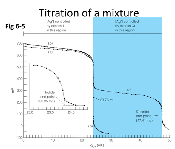
- In the titration curve above (Fig 6-5) 40.00 mL of unknown solution containing I- and Cl- were titrated with 0.0915 M Ag+. What is the concentration of both ions?
STOP
Contributors and Attributions
- Allyson Fry-Petit, California State University Fullerton (afry@fullerton.edu)


