Case Study: Arsenic Analysis

Learning Objectives:

• Identify the details of the various steps in a quantitative analysis method.
• Design a calibration curve using standard solutions of the required analyte.
• Use this calibration curve to calculate the concentration of the analyte in the unknown samples.
• Assess the reliability of the calibration curve and the unknown concentrations using statistical analysis.
• Decide whether the results of the quantitative analysis are sufficient to answer the initial question.

The Problem:

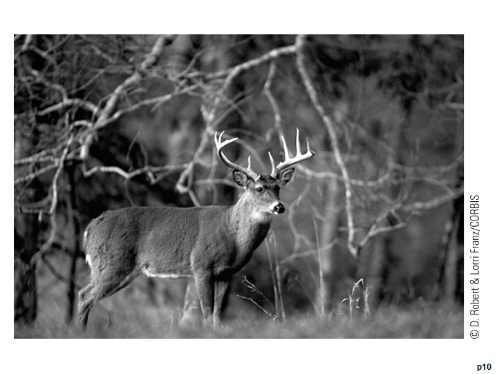
The incident began when a park ranger found a dead white-tailed deer near a pond in the Land Between the Lakes National Recreation Area in western Kentucky.  The ranger enlisted the help of a chemist from the state veterinary diagnostic laboratory to find the cause of death so that further deer kills might be prevented.

The ranger and the chemist carefully inspected the site where the badly decomposed carcass of the deer had been found.  Because of the advanced state of decomposition, no fresh organ tissues could be gathered, and the investigation could not proceed.  However, a few days after the original inquiry, the ranger found two more dead deer near the same location!  The chemist was again summoned to the site of the kill, where he and the ranger loaded the deer onto a truck for transport to the veterinary diagnostic laboratory.  The investigators then conducted a careful examination of the surrounding area in an attempt to find clues to establish the cause of death.

The search covered about 2 acres surrounding the pond.  The investigators noticed that grass surrounding nearby power line poles was wilted and discolored.  They speculated that an herbicide might have been used on the grass.  A common ingredient in herbicides is arsenic in any one of a variety of forms, including arsenic trioxide, sodium arsenate, monosodium methanearsenate, and disodium methanearsenate.  The last compound is the disodium salt of methanearsenic acid (CH₃AsO(OH)₂), which is very soluble in water (as are all salts with cations from Group IA).  Because of its solubility in water, this compound finds use as the active ingredient in many herbicides.

The herbicidal activity of disodium methanearsenate is due to its reactivity with the sulfhydryl (S—H) groups in the amino acid cysteine.  When cysteine in the plant enzymes reacts with arsenical compounds (i.e. compounds containing arsenic), the enzyme function is inhibited and the plant dies.  Unfortunately, similar chemical effects occur in animals as well.  The investigators, therefore, collected samples of the dead grass for testing along with samples from the organs of the deer.  They planned to analyze the samples to confirm the presence of arsenic and, if present, to determine its concentration in the samples.

Selecting a Method:

A scheme for the quantitative determination of arsenic in biological samples is found in the published methods of the Association of Official Analytical Chemists (AOAC).  In this method, the arsenic in the sample is first converted into arsine (AsH₃) and then into a complex ion that has a measurable absorbance in UV-Visible spectroscopy.

Processing the Sample:

1. Obtaining Representative Samples

   Back at the laboratory, the deer were dissected, and the kidneys were removed for analysis.  The kidneys were chosen because the suspected pathogen (arsenic) is rapidly eliminated from an animal through its urinary tract.

2. Preparing a Laboratory Sample

   Each kidney was cut into pieces and homogenized in a high-speed blender.  This step served to reduce the size of the pieces of tissue=e and to homogenize the resulting laboratory sample.

3. Defining Replicate Samples

   Three 10-gram samples of homogenized kidney tissue from each deer were placed in porcelain crucibles.  These served as replicates for the analysis.

Doing the Chemistry:

1. Dissolving the Sample

   To obtain an aqueous solution for the analysis, it was necessary to convert its organic matrix into carbon dioxide and water by the combustion process called dry ashing.  This process involves heating each crucible and sample cautiously over an open flame until the sample stopped smoking.  The crucible was then placed in a furnace and heated at 555^oC for two hours.  This process removes the organic material, leaving behind the arsenic analyte which has been converted into diarsenic pentoxide (As₂O₅).  The dry solid in each crucible was then dissolved in dilute HCl, which converted the As₂O₅ into water-soluble arsenic acid (H₃AsO₄).

2. Eliminating Interferences

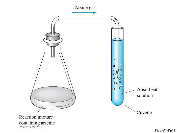
   Arsenic can be separated from other substances that might interfere in the analysis by converting it into arsine (AsH₃), a toxic, colorless gas that is evolved when an aqueous solution of arsenous acid (H₃AsO₃) is treated with zinc.  This is a two-step process: the arsenic acid must be converted into arsenous acid, and then the arsenous acid must be converted into arsine.

   1. The replicate solutions resulting from the deer and grass samples were combined with Sn²⁺ and a small amount of iodide ion was added to catalyze the reduction of H₃AsO₄ to H₃AsO₃ according to the following equation:

      \[\ce{H3AsO4  +  SnCl2  +  2 HCl  →  H3AsO3  +  SnCl4  +  H2O}\nonumber\]

   2. The H₃AsO₃ was then converted into AsH₃ by the addition of zinc metal as follows:

      \[\ce{H3AsO3  +  3 Zn  +  6 HCl  →  AsH3(g)  +  3 ZnCl2  +  3 H2O}\nonumber\]

   This series of reactions was carried out in flasks equipped with a stopper and delivery tube so that the arsine could be collected in an absorber solution.  This arrangement ensured that the interferences were left in the reaction flask and that only the arsine was collected in the absorber in special transparent containers called cuvettes. 

   

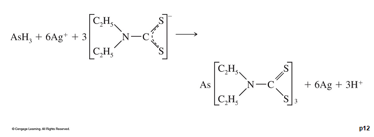
   The absorber solution contained silver diethylthiocarbamate, which forms a red complex with arsenic:

   

 

Measuring the Amount of Analyte:

The amount of arsenic in each sample was determined by measuring the absorbance of each sample with a UV-Vis spectrophotometer.  The absorbance is proportional to the concentration of the analyte, so the concentration of the analyte can be determined using Beer’s Law and a Least-Squares Analysis.  In order to determine the concentration of the analyte, a calibration curve must be generated using a series of standard solutions containing known amounts of the analyte.

Since the arsenic in the kidney tissue of an animal is toxic at levels above about 10 ppm, the standards were chosen in the 0-25 ppm range:

Arsenic Concentration (ppm)	Absorbance
0.0 (blank)	0.00
5.0	0.13
10.0	0.28
15.0	0.42
20.0	0.59
25.0	0.71
Deer #1 (unknown concentration)	0.47
Deer #2 (unknown concentration)	0.63

Now It’s Your Turn:

Instructions:  Show all of your work for each of the calculations below (Problems 2-8).  These calculations must be presented in an orderly fashion with all correct units and significant figures in the final answer.  End each of these problems with a detailed sentence explaining what you learned.  Please attach these calculations to the paper copy of your spreadsheet, and email an electronic copy of only the spreadsheet to me.

1. Using an Excel spreadsheet, plot the data for the calibration curve. Use an xy-scatter plot, and tell it to plot the best-fit straight line.

 

2. Using the statistical equations from Chapter 8, calculate the least-squares slope and y-intercept, and then write the equation for your best-fit line.

 

3. Calculate the standard deviation about regression, and tell me what it means.

 

4. Calculate the standard deviation for the slope and for the y-intercept, and report a final value for each of these quantities that includes its standard deviation (i.e. value ± std dev). Tell me what the standard deviation tells you about the precision of each quantity.

 

5. Using the equation for the best-fit line, calculate the concentration of arsenic in both of the unknown deer samples.

 

6. For both of these unknown deer samples, calculate the absolute standard deviation and the coefficient of variation.

 

7. Repeat the calculations in (6), assuming that the absorbance reading for each unknown was the mean of three replicate absorbance readings.

 

8. Calculate the coefficient of determination (R²) for this best-fit line, and tell me what it means.

 

9. Annotate the flow diagram showing the steps in a quantitative analysis with specific details from this particular case study.

 

10. Are the results of this quantitative analysis sufficient to answer the initial question? Explain.

 

Contributors and Attributions

• Sheri Strickland, Converse College ([e-mail])
• Based on the case study Deer Kill from Fundamentals of Analytical Chemistry, 9^th edition, Chapter 1
• Sourced from the Analytical Sciences Digital Library