Calibration Methods (Gray)

Learning Objectives:

At the conclusion of this activity, students will be able to:

1. Explain the differences between external standard and standard addition calibration and describe situations when each should be used.
2. Give examples of when an internal standard is necessary and describe what types of experimental error it can correct for. 
3. Calculate the concentration of an analyte given raw data using any of these calibration methods (external standard, standard addition, internal standard).
4. Determine which method is most appropriate to utilize when faced with a real world analytical problem. 

Why does concentration matter? Why must we calibrate?

Accurately knowing the amount, in terms of concentration, of a particular substance (analyte) is important in fundamental research and also in many applied fields of study.

In order to determine the concentration of a particular analyte in a sample using a specific instrument we must perform a procedure called “concentration calibration.” While analytes themselves cannot be measured directly, specific properties of the analyte are measurable. Many analysis techniques provide a response (signal) to a solution containing some concentration of an analyte. For example, the light absorption properties of a chemical may be measured to determine its concentration in a sample. Calibration is the process of determining the sensitivity of an instrument to a particular analyte, or the relationship between the signal and the amount of analyte in a sample.

Q1. As a group, devise a way in which you could determine how the signal from an unknown concentration of analyte corresponds to its concentration.

 

 

 

 

 

 

 

External Standard Calibration

To determine the concentration of 2,3-butanedione (diacetyl, boiling point 88 °C) in beer, a headspace gas chromatography method is utilized. A series of standard solutions are created to define the instrument response to varying concentrations of analyte.

Specifically, a stock solution is created by adding a specific amount of diacetyl primary standard to a solution of 5% (v/v) ethanol in water. This stock solution is then diluted to give a series of lower concentrations of the analyte; this is most commonly done using the serial dilution method as shown below. For the dilution of diacetyl, an aliquot of the stock solution is transferred into a new volumetric flask, diluted (with 5% ethanol in water) and mixed well to produce diluted solution 1. Then, the same aliquot amount from diluted solution 1 is transferred into a new volumetric flask, diluted to the mark, and mixed well to prepare diluted solution 2.  The process is repeated in this manner until a series of solutions have been prepared in which each successive solution is more dilute than the previous. The figure below illustrates preparation of three dilutions starting with the stock solution.

Calculations are performed using the dilution equation:  \(\mathrm{C_1V_1 = C_2V_2}\)

Where C is concentration, V is solution volume, and the subscripts 1 and 2 refer to the initial solution and the more dilute final solution, respectively.

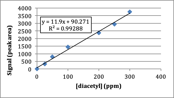
When each standard, along with a blank (no diacetyl added), is run on the gas chromatograph, a signal (peak area) is recorded for each concentration of diacetyl, as given in Table 1.

Diacetyl (ppm)	Signal (peak area)
0	0
25	330
50	793
100	1442
200	2367
250	2945
300	3762

Table 1. Signal generated for each standard solution of diacetyl.

Figure 1. Plot of the concentration of diacetyl vs. peak area signal for headspace analysis of diacetyl in beer.

Q2. Does the regression line in the external curve plot fit the data well? How did you determine if the fit was good?

 

 

 

 

 

Q3. Use the equation information generated in Figure 1 to calculate the concentration of diacetyl that would yield a peak area of 2598.

 

 

 

 

The general steps involved in using standard analyte concentration and detector response data to calculate an unknown analyte concentration using linear regression and the method of least squares is as follows:

1. Create a scatter plot of the data
2. Create a linear regression line (trend line)
3. Obtain a regression equation and R-squared value
4. Rearrange the regression equation to calculate the unknown analyte concentration

Q4. Referring to the calibration curve in Figure 1, what could be done to obtain the concentration of diacetyl in a solution that has an signal beyond the linear range of the calibration curve (for example, a peak are of 4519)?

 

 

 

 

 

Internal Standards

For the determination of diacetyl using headspace gas chromatography, the standards and beer samples are heated in special vials at 60 °C for 45 min. Once heated, a 500-μL sample is collected from the headspace of each vial using a gas-tight syringe and injected onto the instrument.

Q5. What is the purpose of heating the samples?

 

 

 

 

 

Q6. List the factors that may impact the amount of diacetyl collected in the syringe and injected onto the instrument.

 

 

 

 

 

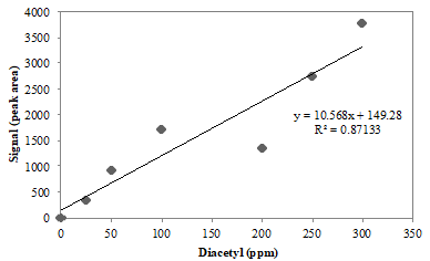
A research student runs diacetyl standards and constructs the following calibration curve:

Figure 2. Calibration curve for diacetyl standards run using headspace gas chromatography. The instrument response (signal) is given as peak area, which is proportional to concentration.

Q7. Describe the relationship of the data points to the trend line in Figure 2. Does the trend line adequately fit the data?

 

 

 

Q8. Should the calibration curve in Figure 2 be used to calculate the concentration of diacetyl in the beer samples? Why or why not?

 

 

 

Q9. As a group, brainstorm a way you could correct for the error observed in the Figure 2 calibration curve.

 

 

 

An internal standard (I.S.) in analytical chemistry is a substance similar to the analyte that is added in a constant amount to the blank, the standards, and the samples. They are useful to compensate for changes in extraction efficiency, detector response due to sample loss during other sample preparation steps, fluctuations in sample analyzed, or changes in detector response due to different flow rates. Internal standards are widely used in chromatography because of differences in the reproducibility of sample injected into the chromatograph. All of these changes should affect the internal standard to the same degree as the analyte so that the relative ratio of the standard to analyte remains constant.

For the quantification of diacetyl in beer, 2,3-hexanedione is most commonly utilized as an internal standard.

Q10. Draw the chemical structure of diacetyl (2,3-butanedione) and 2,3-hexanedione. What are their boiling points?

 

 

 

 

 

 

Q11. Based on your answer to Q11, would 2,3-hexanedione be a good choice as an internal standard for the analysis of diacetyl? Why or why not?

 

 

 

 

 

 

In a gas chromatography experiment, a standard solution containing 25 ppm of diacetyl, represented by X, and 0.05 ppm of internal standard 2,3-hexanedione, represented by S, give peak areas of A_x=330 and A_s=59 (areas in arbitrary units), respectively.  The response factor or response ratio (F) can be calculated using the following equation and rearranging the equation to solve for F:

\[\dfrac{Ax}{[X]}=F\left(\dfrac{As}{[S]}\right)\nonumber\]

F must be determined by measuring known concentrations of both diacetyl and 2,3-hexanedione first, before you can use this equation to determine an unknown concentration of diacetyl. If a calibration curve is created, one must determine the signal from both the analyte and internal standard and plot the relative signal vs. the concentration of the analyte standard, as shown in the data in Table 2.

Diacetyl (analyte, ppm)	2,3-hexanedione (I.S., ppm)	Analyte peak area	I.S. peak area	Signal ratio (analyte/I.S.)
0	0.05	0	58
25	0.05	330	59
50	0.05	911	82
100	0.05	1720	74
200	0.05	1352	28
250	0.05	2745	48
300	0.05	3762	55

Table 2. Signal collected for 2,3-butanedione samples spiked with a 2,3-hexanedione internal standard.

Q12. Calculate the signal ratio for each standard and fill in the results in the empty columns of Table 2. Calculate F for the 25 and 50 ppm standards. Are the F values similar/different?

 

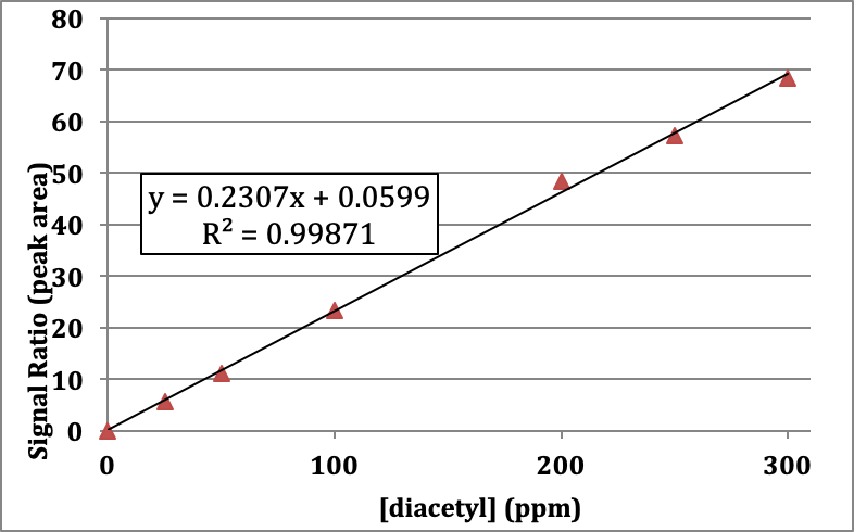
Q13. If you want to construct a calibration curve for diacetyl incorporating the internal standard, what should be plotted on each axis? When finished, check your work with the instructor and ask for a copy of the new calibration curve.

 

Q14. Describe the relationship of the data points to the trend line for the calibration curve your instructor provided. Does the trend line adequately fit the data?

 

Q15. A beer sample spiked with 0.05 ppm internal standard has a diacetyl peak area of 1497 and an I.S. peak area of 63. What is the concentration of diacetyl in the beer?

 

Q16. When is an internal standard needed in a calibration method?

 

 

Standard Addition

For many analytical methods it is possible to run an external calibration, as described above. There are situations however where this approach does not work well.

A common problem that can occur in chemical analysis is known as a matrix effect.  The matrix is everything else in the sample except the analyte.  Components of the matrix may interact with the analyte and alter its response in the measurement technique.  Matrix effects can sometimes enhance the response, whereas other times they can decrease the response.  For example, when analyzing lead in soil there may be other chemicals present that will affect the signal for lead.  Since the components that make up the soil matrix are often complex, not completely known, and possibly vary from sample to sample it would be impossible to replicate these matrix effects in an external standard.  

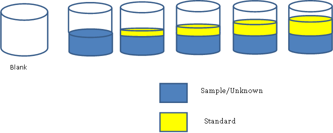
The standard addition method is similar to the external calibration method in that the concentration of an analyte is determined by comparison to a set of standard solutions of the analyte.  However, in the standard addition method, the standard is added directly to the sample (same flask) to correct for ‘matrix effects’ (a change in the analytical signal caused by anything in the sample other than the analyte).  This is called “spiking.”  This can be done for a single sample or for multiple samples. The figure below shows how samples could be made to create a standard addition calibration curve.

Figure 3. Example of how to create solutions for a standard addition calibration curve.

Single Sample:

The single sample method described here is a 1-point calibration. While not ideal, this may be necessary if you have a limited amount of your unknown sample (especially if your analysis method is destructive).

Note:

If your analysis method is non-destructive, you can add an aliquot of standard to the unknown, measure it, and continue to add aliquots of standard to create a standard curve. We will not be considering this method here.

When standard addition is performed with only one sample, the sample is analyzed alone and then reanalyzed after the standard addition is performed.  Once the spike has been performed, the total concentration of the analyte (from the standard addition and from the sample) is directly proportional to concentration.

\[\dfrac{\textrm{Concentration of analyte in initial solution}}{\textrm{Concentration of analyte plus standard in final solution}} = \dfrac{\textrm{signal from initial solution}}{\textrm{signal from final solution}}\nonumber\]

\[\textit{Standard addition equation:} \hspace{40px} \dfrac{[X]_\textrm i}{[S]_\textrm f + [X]_\textrm f}  = \dfrac{I_\textrm X}{I_\textrm{S+X}} \tag{5-7}\]

In the equation above X represents the concentration of analyte from the unknown sample and S the concentration of analyte from the standard. It is important to remember that with standard addition these are chemically the same species.  You also must keep in mind that when the standard addition solution is added to the sample the sample is diluted. The i subscript in the equation above stands for initial or the concentration of the analyte before the standard spike is made.  The f stands for final which is the concentration after the spike has been added.

Note:

Since you are solving for [X]_i, the equation takes into account the dilution from adding the sample. If the volume of unknown added was from an original (undiluted sample), you don’t need to do any further calculations to determine the original concentration.

Researchers can use the amount of strontium in tooth enamel found in archeological specimens to understand more about ancient cultures and diets.  A 10.0 mL sample is prepared by dissolving 0.750 mg of tooth enamel and analyzed by atomic absorption spectroscopy.  This analysis gives a signal of 28.0 units.  Next 5.00 mL of the original sample is combined with 2.00 mL of standard strontium solution that has a concentration of 25 ng/mL.  This new sample is diluted to a final volume of 10.00 mL and analyzed by AA spectroscopy.  The sample with this standard addition has a signal of 42.8 units.

Q17. What is the concentration (ng/mL) of strontium from the standard addition spike in the second sample analyzed (find [S]_f)?

 

 

 

 

 

Q18. Plug the given numbers and the number you calculated in Q17 in equation (5-7) and show it below. (Don’t solve the equation yet)

 

 

 

 

 

 

At this point you have one equation with two unknowns so you cannot solve it as is.  However there is a relationship between [X]_i and [X]_f.

Q19. Write an equation showing the relationship between [X]_i and [X]_f.

 

 

 

 

 

 

 

Q20. Combine the equations from questions Q18 and Q19 to get an equation with only one unknown [X]_i.

 

 

 

 

 

 

Q21. What was the concentration of strontium (ng/mL) in the sample ([X]_i)?

 

 

 

 

 

 

 

 

 

 

 

Q22. What is the concentration in ppm of strontium in the tooth enamel analyzed?

 

 

 

 

 

 

 

 

Multiple samples/solutions:

When using a calibration curve, increasing amounts of analyte are added to a constant amount of sample.  The concentration of the analyte is then obtained by extrapolating back to the x-intercept; the absolute value of the x-intercept is the concentration of the measured sample of unknown as shown below:

Figure 4. Description of a standard addition calibration curve.

If the sample was diluted prior to measurement, you need to manually un-do the dilution to get back to the original concentration of the solution.

Lead in river sediment is measured using the technique of standard addition.  The chart below shows the signal from a diluted unknown sample and the signals obtained by adding increasing amounts of standard to the sample. To make the diluted unknown sample, 5.50 mL of the unknown were added to a 25.0 mL volumetric flask, which was diluted to the mark with DI water. The graph is shown below.  Use the equation to answer the question below.

Concentration of lead standard in the sample (ppb)	Signal
0	1.10
2	1.66
4	2.20
6	2.81
8	3.41
10	4.00
15	5.51

Table 3. Concentration of lead standard added to a river sediment sample and the corresponding instrument signal.

Figure 5. Standard addition calibration curve for the analysis of lead in river sediment.

 

Q23. Calculate the x-intercept of the graph shown (include units).

 

Q24. What does the value you found in Q17 mean?

 

 

 

Q25. What is the concentration of lead in the original unknown?

 

 

 

 

Q26. When is the standard addition calibration method needed?

 

Q27. What would Figure 3 look like if you used an internal standard with the multiple solution standard addition calibration method?

 

 

 

Calibration Methods

Figure 3. Calibration curve for diacetyl standards + an internal standard (2,3-hexadione) run using headspace gas chromatography. The instrument response (signal) is given as a ration of the peak area of the analyte to the peak area of the internal standard, which is proportional to concentration.

 

 

 

Calibration Methods-Applications

Name:_____________________________

Case Study 1:

A scientist wants to measure the amount of vitamin C in an energy bar.  The bar is ground up and dissolved in an organic solvent.  An extraction is then preformed with water.  Vitamin C is very water soluble and is expected to be found in the aqueous layer after the extraction many of the other bar components especially the fats remain in the organic.  The aqueous layer is then analyzed to determine vitamin C content with an external standard curve.  When multiple energy bars are analyzed the results have poor precision and often less vitamin C is recovered then was expected.

What are the sources of error in this experiment?

 

 

 

Suggest improvements to this experiment.

 

 

 

 

 

Case Study 2:

A scientist wants to develop a new assay to determine the amount of a banned substance in the blood of athletes.  The new assay is faster and cheaper than the old assay, but the results in some samples of blood are higher than with the old assay leading to false positives for some athletes.  The new assay utilizes external calibration.  If a single sample is run multiple times, the precision is acceptable even for the false positive samples.

What could be causing these false positives?

 

 

 

Suggest improvements to this experiment to eliminate these false positives.

 

 

 

Contributors and Attributions

• Sarah Gray, Stockton University ([e-mail])
• Adapted from materials by:
  • Dr. Rebecca A. Hunter, The Citadel
  • Dr. Amanda Harris, Virginia Commonwealth University
• Sourced from the Analytical Sciences Digital Library