3.2: Biochemistry

Isolation and Purification of Glycinamide Ribonucleotide Synthetase, the second enzyme in the purine biosynthetic pathway

Background

Enzymes are proteins that catalyze reactions 10⁶ to 10¹⁵ times the rate of the same uncatalyzed reactions. The detailed analysis of the mechanism by which these tremendous rate accelerations occur has intrigued biochemists for decades. Recently Cech and his coworkers discovered that ribonucleic acids (RNAs) can also catalyze reactions of biological importance. The vast majority of catalysts inside cells, however, are protein molecules. This module will focus on teaching you techniques essential for working in any biochemistry lab. You will learn how to purify a protein which has been genetically engineered to facilitate its purification. You will characterize the protein using electrophoretic methods and by standard steady state kinetic methods. The three dimensional structure of this protein has recently been determined at atomic resolution and you will examine this structure in an effort to establish which amino acid side chains in the active site would be worth changing to investigate their role in catalysis. Several mutant genes have already been made in the Stubbe lab. You will express the wild type or a mutant protein and determine its kinetic parameters. Using the structural information and a comparison of the kinetic parameters of the wild-type and mutant proteins (the data for the entire class will be analyzed), you will propose a chemical explanation for these results.

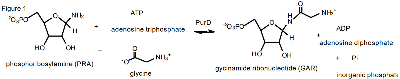
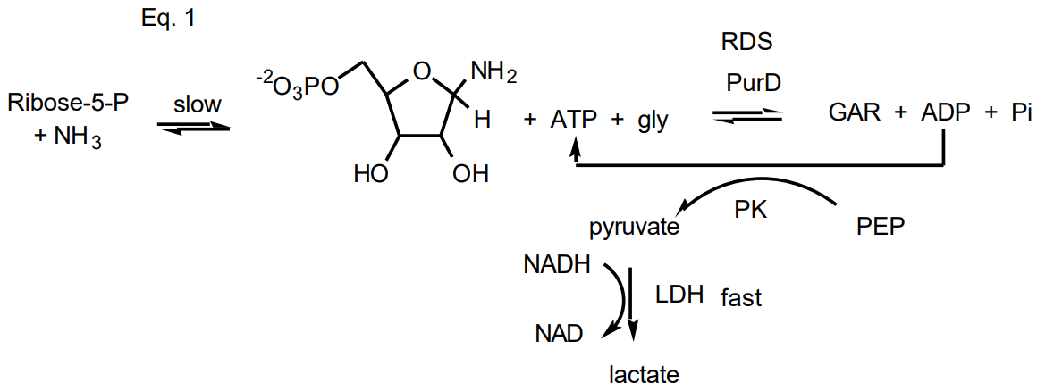
The protein we have chosen to investigate is glycinamide ribonucleotide (GAR) synthetase which catalyzes the conversion of phosphoribosylamine (PRA), adenosine 5'-triphosphate (ATP) and glycine (G) to GAR, adenosine 5'-diphosphate (ADP) and inorganic phosphate (Pi) (Figure 1). GAR synthetase is also called by its gene name PurD. This is the second enzyme in purine biosynthetic pathway, Figure 2. ATP is proposed to phosphorylate the carboxylate of glycine to generate a phosphoanhydride that is activated toward nucleophilic attack by the amino group of PRA. The GAR synthetase reaction is reversible with a Keq of 15.

Recently the 3-dimensional structure of the protein was solved at atomic resolution and this structure established that the protein is a new member of the ATP grasp superfamily of proteins most of which catalyze similar chemistry to that proposed for GAR synthetase. However, both the substrate to be phosphorylated and the nucleophile acceptor differ widely among members of this superfamily (Table 1).

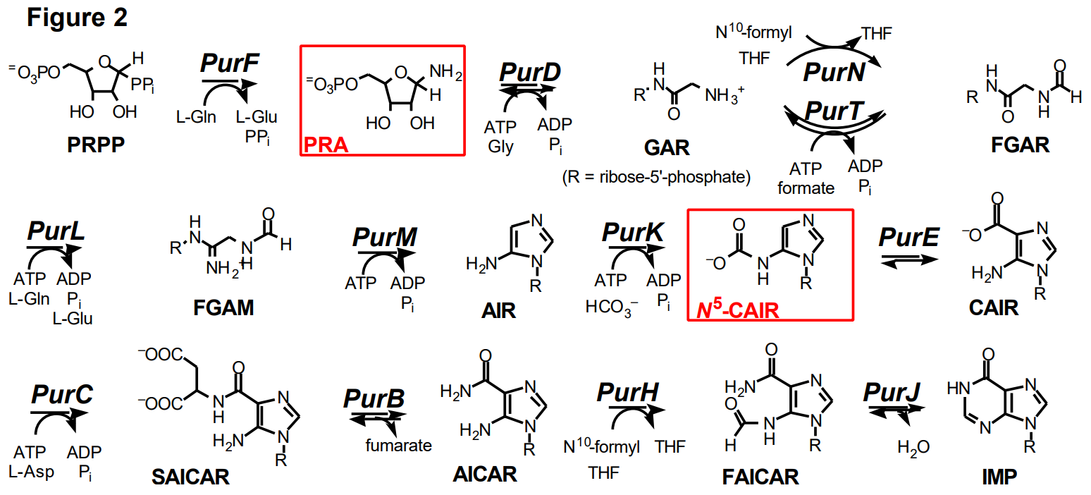
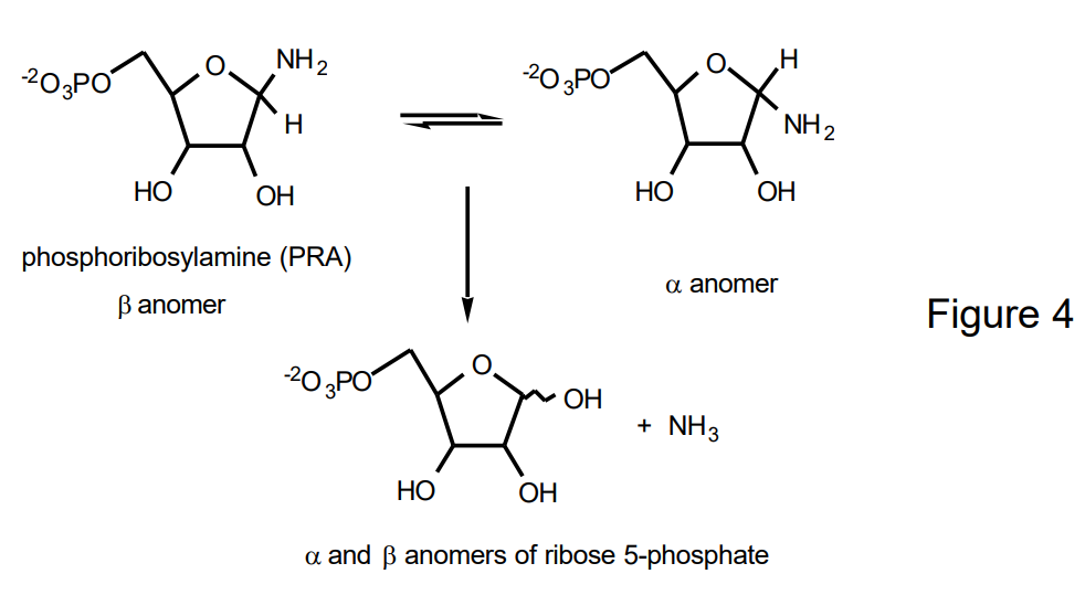
GAR Synthetase is of interest from a biochemical viewpoint for a number of reasons. PRA, its substrate, is chemically unstable having a half life of 15 sec at pH 7 and at 4°C. PRA rapidly hydrolyzes to ribose-5-P and ammonia (Figure 4) and rapidly anomerizes to give a 3:2 mixture of \(\beta :\alpha\) anomers. The question can be raised as to whether PRA, produced by the first enzyme in the purine biosynthetic pathway, phosphoribosylpyrophosphate amidotransferase (PurF, Figure 2) directly

Table 1 ATP Grasp Superfamily Members

Name of Enzyme	Reaction
D-ala-D-ala ligase	2 alanine + ATP = D-alanine-D-alanine + ADP + Pi
glutathione syn	gly + ATP + glucys = glutathione + ADP + Pi
PurK	aminoimidazole ribonucleotide (AIR) + ATP + HCO3^- = the carbamate of AIR + ADP + Pi
PurT	glycinamide ribonucleotide (GAR) + ATP +formate = formyl-GAR (FGAR) + ADP + Pi

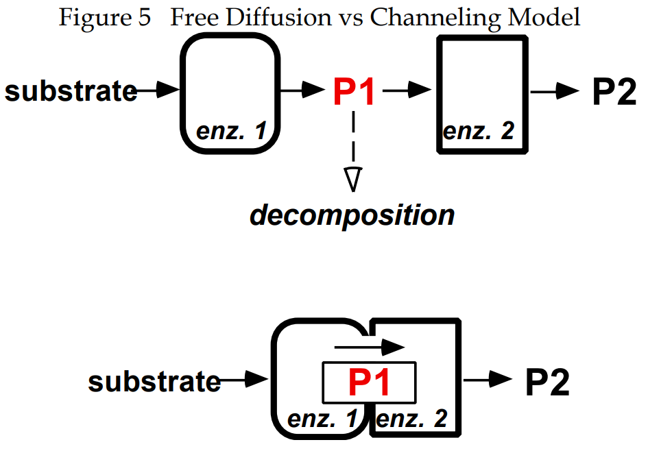
transfers (channels) its product to GAR synthetase (PurD) or whether PRA (P1, Figure 5) dissociates into solution subsequent to its formation by PurF and is then picked up by GAR synthetase.

The protein is also of interest as three other enzymes (Pur T, PurK and PurC, Figure 2) in the purine biosynthetic pathway catalyze similar reactions. When thinking about the evolution of a biosynthetic pathway, one wonders whether these proteins that catalyze similar chemistry, will also be structurally similar. PurK, PurT and PurC structures have recently been solved and they are all members of the ATP grasp superfamily.

 

Protein purification:

The revolution in molecular biology has greatly facilitated purification of proteins, at least from procaryotic systems. The gene for PurD (purD) has been engineered as described below to contain a hexa histidine tail tag at its N-terminus. This engineered construct has been placed in a plasmid containing a T7 promoter in a pET vector obtained from Novagen. Genes for proteins placed behind T7 promoters produce RNA only in the presence of a T7 RNA polymerase not normally found in host E. coli. Certain E. coli host strains, such as E. coli BL21(DE3), have therefore had a T7 RNA polymerase integrated into their genome and this polymerase is under the control of the lac promoter which is inducible in the presence of isopropyl thio-\(\beta\)-galactoside (IPTG) . In the construct that you were given for the expression of PurD, IPTG addition results in the induction of PurD so that it constitutes about 25% of the total protein in the cell, greatly facilitating its purification. However, the protein is also generated in substantial amounts in the absence of IPTG due to the leakiness of the promoter. In the induced growth system, one in four of the proteins in the crude cell extract is the PurD, in contrast to one in 500-1000 which is more typical for purification of the protein from BL21(DE3) which produces PurD under its normal growth condtions. As you can imagine, the increase in the amount of the desired protein greatly facilitates its purification.

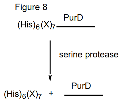
One of the most popular methods to purify proteins is the addition of a oligohistidine peptide linker at either the N or C-terminus of the protein of interest. This tail, if accessbile to the outside of the protein can form a complex with a column that contains imino di or triacetic acid bound to a metal in the +2 oxidation state, such as Co²⁺ or Ni²⁺. The tail of the protein of interest chelates to the metal and is retained on the column. Most of the other proteins in the E. coli crude cell extracts are washed through the column. The protein of interest is then eluted with imidazole or ethylenediamine tetraacetic acid, EDTA. Each of these species competes with the histidine linker at the end of the protein for complexation with the metal. Often times the His linker is placed adjacent to a stretch of 7 specific amino acids ( in a nonstructured, protease specific sequence) which are recognized and accessible to a commercially available serine protease such as thrombin (Figure 8). In this fashion, the histidine-tagged protein of interest, once purified, can be cleaved from the protein by brief incubation with the serine protease. It should be noted, however, that the activity of many proteins isolated in the last few years appear to be unaltered by the attachment of a hexahistidine tail and consequently in many cases no effort is made to remove the tag. In the case of GAR synthetase the specific activity of the enzyme in the presence and absence of the tag is 19 units/mg [a Unit is the number of mmoles of product produced per min] and 42 units/mg, respectively. In fact the published crystal structure of GAR synthetase is of a protein with such a linker. The linker is not visible, that is, it is not detected crystallographically because of its thermal lability. The N-terminus is located on the surface of the protein.

 

Protein Purification and Characterization:

Session 1: Preparation of Reagents, Learning Sterile Technique and Use of the Pipettemen and Spectrophotometer.

You will first sterilize media for bacterial growth. You will then make a standard curve using bovine serum albumin and use this curve to determine the concentration of an unknown protein solution that will be given to you by the TA. At the end of the class you will be given a 5 mL culture of E. coli that contain the plasmid with PurD. You will inoculate 250 mL of your sterilized media and let your bacteria grow overnight.

 

Instrument Use: 

Instructions for Reading Absorbance Using the Varian Cary 100 Spectrophotometer

1. Turn on the spectrophotometer.
2. Open the “Simple Reads” program, which can be found on the desktop icon, or under the Cary WinUV menu through the “Start” button.
3. The lamps are on if under the “Commands” menu you see “Lamps Off.” If you see “Lamps On,” click this to turn on the lamps. For accurate measurements, the lamps require 15 minutes to warm up. 
4. To setup the instrument, click the “Setup …” command button on the left side of the screen. In the “Read at Wavelength” scroll box, type in the desired wavelength. The “Abs” button in “Y mode” should be selected. When you are finished with setup, click the “OK” button to exit the window.
5. Before you can measure the absorbance of your sample, you must zero the instrument. Open the lid and determine which cell is in the light path. Insert a cuvette with your blanking solution in the instrument. The blank solution should be identical to your sample solution, but without the analyte. Close the lid completely, and press the “Zero” command button on the left side of the screen to zero the instrument at your chosen wavelength. The blank should have an absorbance of zero now, but notice that there is a small amount of “noise” present at all times.
6. You are now ready to read the absorbance of your sample. Insert a cuvette containing your sample into the instrument, close the lid completely, and press the “Read” command button at the top of the screen. The absorbance of your solution should be recorded on the screen.
7. Under the “File” menu, select “Print” to print your data.
8. When finished, close the program to return to the desktop. 
9. Turn off the lamps, then turn off the instrument.

 

Use of the Autoclave

(Use of this instrument will be demonstrated by the TA. The details of the use are posted adjacent to the instrument)

 

Preparation of Solutions

Media:

LB (Luria-Bertani) medium is 1% bacto-tryptone, 0.5% yeast extract and1.0 % NaCl. All of these measurements are weight/volume (w/v), measured as g/100 mL. This LB comes premixed and you use 25g/L, just as the calculation predicts. You have to transfer, using sterile technique demonstrated by the TA (See Appendix p. 45), 250 mL of sterilized LB into a 1 L flask. The TAs have prepared a solution of kanamycin (70 mg/mL) which has been filter sterilized. You will need to add 0.25 mL of this solution to your cooled, sterilized media. You will then inoculate this flask with 5 mL of bacteria grown overnight from a single colony, also prepared by the TAs. The flask will then be placed in a 37 °C shaker and the bacteria grown overnight with shaking and collected the following day. Each pair of workers will be given bacteria with a plasmid which contains the gene for wild type or a mutant PurD. If you are given a mutant of PurD, the sequence of your mutant is recorded in a notebook kept by the head TA.

Reagents to prepare:

For use in the determination of the protein concentration by the procedure of Lowry.

Make 10 mL of a 1.0 mg/mL aqueous solution of bovine serum albumin (BSA). SAVE THIS STOCK SOLUTION FROZEN in 1 mL aliquots at -20°C AS YOU WILL USE IT TO DETERMINE PROTEIN CONCENTRATIONS THROUGHOUT THIS MODULE. This protein solution will be used for preparation of the standard curve for determining the concentration of protein throughout the course of the module. While you will weigh the BSA on a balance, in biochemical experiments, frequently weight is not the most accurate way to establish a concentration. In the case of BSA, the extinction coefficient at 280 nm is established to be 0.67(mg/mL)^-1. You need to measure the actual concentration of BSA using a quartz cuvette and the spectrophotometer. How does this value compare with what you thought you weighed? Why is the \(\lambda\)max of BSA at 280 nm?

Lowry Reagents for Protein Determination:

Lowry A solution: Prepare one liter of a solution containing 20g of Na₂CO₃, 4g of NaOH and 0.2g of sodium tartrate.

Lowry B solution: Prepare 100 mL containing 0.5g of CuSO₄•5H₂O.

Lowry C is made directly before use and is composed of 50 mL of Lowry A and 1 mL of Lowry B.

The final reagent is the phenol solution which is composed of 25 mL of Folin and Ciocalteu reagent (2N phenol) mixed with 35 mL of H₂O.

Preparation of a Standard Curve using BSA:

In 8 separate 1.0 mL Eppendorf tubes label and add: 200 µL of your stock BSA solution+ no water; 150 µL BSA + 50 µL water; 125 µL BSA + 75 µL water; 100 µL BSA + 100 µL water; 75 µL BSA + 125 µL water; 50 µL BSA + 150 µL water; 25 µL BSA + 175 µL water and 200 µL of water. In 8, 1.5 mL Eppendorfs add 1 mL of Lowry reagent C and 100 µL of each of the above protein solutions. Mix each solution using the Vortex apparatus. Then add 100 µL of phenol reagent to each Eppendorf and mix well. Wait for 30 min and then read the absorbance at 670 nm using the no protein sample as the reference. Absorance at 670 nm should be read in a plastic rather than a quartz cuvette. Why? Plot your data A_670nm vs mg/mL of BSA to establish that you can reproducibly obtain a straight line.

Note

You will be use the Lowry method with BSA numerous times to determine your protein concentration during the purification of PurD. If your line is straight in the above experiment, you can cut back to 5 concentrations to prepare your subsequent standard curves. You will be given by the TA a protein solution of unknown concentration.

You will use your standard curve to determine the concentration of this solution. NOTE You should use a range of concentrations for your unknown to ensure that your A670 nm will reside on the linear portion of your standard curve. You should use several samples (2-3) of the unknown at different concentrations to correctly determine the BSA concentration.

 

Session 2:

This session may take two afternoons. Learning the Use of the Centrifuge, pH meter, end point assay for determination of the concentration of PRA, protocol for assaying GAR synthetase activity, preparation of the Ni-Affinity column and reagents required for PurD purification.

You will be given a known amount of PurD and you will determine its specific activity. The specific acitivity you determine will be turned into the TA when the session is completed. You will not be allowed to proceed to the next section until you have determined this value correctly.

Instrumentation:

The TAs will demonstrate the use of the centrifuge and pH meter. It is important to calibrate the pH meter before use.

Isolation of Bacterial Cells that contain GAR synthetase:

Remove the culture from the 37°C shaker and cool it in an ice bucket to stop the growth. Place the culture into a 500 mL centrifuge tube. Balance your bottle and its cap, using a swinging balance, with a tube and cap prepared by your neighbor. Centrifuge the cells at 6,000 rpm (3,950 x g) for 10 min at 0°C using the JA-10 rotor in the Beckman J2-HS centrifuge or the GSA rotor in the Sorvall. The TA will demonstrate how to use the centrifuge. After pelleting the cells, carefully decant (pour off) the supernatant into the original flask. Add Clorox bleach to the supernatant in the flask to a final concentration of 10%. This procedure kills any remaining bacteria. Using a wooden tongue depressor transfer the pellet to a preweighted falcon tube and reweigh the tube to determine the number of grams of cells harvested. Record this number in your notebook. Freeze the cell pellet at -20°C for use in Session 3.

Preparation of Solutions:

The solutions that you prepare are the key to successful experiments. In many cases the biological molecules are unstable. One needs to understand their chemical properties to make sure that the compounds are stored in solution at the appropriate pH and temperature. A list of the reagents, molecular weights and storage conditions are in the Appendix p. 44. Make sure that the molecular weights agree with the reagents on the shelf. In addition to pH, determining the concentrations of certain biological compounds is more complex than weighing your material and dissolving it in a given volume of water or buffer. Biological molecules are often hygroscopic and the weight will vary depending on the amount of moisture in the air. If the biological material of interest is chromophoric, the concentration should be determined by measuring its absorption as a function of wavelength. You have already done this with BSA in the previous session. Using the known extinction coefficient(\(\epsilon\)) of the compound of interest at a given pH and Beer's law, the concentration can be determined. Often times the biological molecule may not be chromophoric and therefore you need to be creative about determining its concentration. Often you will convert the compound of interest into a species that is chromophoric and whose extinction coefficient is known. If you use this approach, you must make sure that the conversion of your compound to the chromophoric species is quantitative.

Preparation of Solutions: A large number of solutions need to be prepared. The TAs will make assignments to each team for the preparation of a given solution. These solutions will be used by all of your classmates, so that it is essential that your solution be prepared correctly. Each team will prepare their own assay solutions (except for NADH, 5 M Imidazol, Coomassie Stain, Destain Solutions, Lamelli Buffer, Gel Fix, and PEP which will be prepared by the TAs) . The TAs will provide you with a stock solution of 0.5M EDTA, pH 7.5. These solutions will be used throughout the remainder of the module.

The Roman numerals (I, II etc) indicate that group I will prepare these solutions, group II etc. A * indicates that the solution will be prepared and given to you by the TA. The assignment for solution preparation will be made by the TA.

1. Lysis Buffer:  The lysis buffer (250 mL) contains 50 mM Tris, 1 mM EDTA and 100 mM NaCl. The solution needs to be cooled to 4°C and then adjusted to pH 8.0 with 1 N HCl (obtained from the TAs). Be careful to calibrate the pH meter at 4°C as well. Tris has the unpleasant property that its pH is very temperature dependent. You should convince yourself that this is true by measuring the pH of your buffer at room temperature. Dilute your sample to 250 mL using a volumetric flask. Each student will use 3 mL of this solution per gram of bacterial cells they isolate. This 250 mL of solution should thus be sufficient for use by the entire class.
2. Stock solutions for use with the Ni Affinity column to be used in the purification of GAR synthetase: 
   1. Preparation of the Ni-affinity column: 10 mL of 0.1 M NiSO4 
   2. Washing the Ni-affinity column: 1 L of 50 mM Tris which is adjusted to pH 7.5 with 1 N HCL (obtained from the TAs) and the solution must be cooled to 4°C.
   3. You will also use a 10 mL stock solution of 5 M imidazole at pH 7.5. This has been made by the TAs. The pH of the solution needs to be adjusted with concentrated HCl obtained in the fume hood. Add the HCl dropwise so that you don't overshoot the desired pH. Check the pH with pH paper. This stock solution will be used to make up a buffer composed of 50 mM Tris (pH 7.5) in 5 mM imidazole to wash your Ni-affinity column. [Note: since your imidazole solution must be diluted 1 to 1000, you do not need to worry about the dilution of your Tris solution when making it 5 mM in imidazole.]
3. Dialysis stock buffer solution: 1 L of 0.5 M Tris, pH 7.8 at 4°C. The pH should be adjusted with concentrated HCl.
4. Preparation of Solutions for 12 % Sodium dodecyl sulfate polyacrylamide gel electrophoresis (SDS PAGE) gels: These solutions can be used by the entire class.
   1. Running buffer: Prepare 2L of 5X running buffer with 15.1 g/L of Tris, 72 g/L of glycine and 5 g/L of SDS
   2. Coomasie for Staining your SDS PAGE gel: Make 500 mL and this stain can be used by the entire class. 0.05% Coomasie blue, 50% methanol, 10% acetic acid, 40% water. The TAs should prepare this solution.
   3. Fast Destain Solution: 1L, This solution allows destaining in 1-3 hours. 40% (v/v) methanol and 10% glacial acetic acid. The TAs should prepare this solution. Slow Destain Solution (for destaining overnight): 1L, 10% glacial acetic acid, 5% methanol. The TAs should prepare this solution.
   4. 4X upper gel (stacking) gel buffer: 6.05 g Tris and 0.4 g SDS which should be adjusted to pH 6.8 and then diluted to a final volume of 100 mL. The solution should should be stored at 4°C.
   5. 4X lower gel buffer: 91 g Tris, 2g SDS and the pH adjusted to 8.8 and the solution then diluted to 500 mL. The solution should be stored at 4°C.
   6. 2X Lamelli Gel loading buffer: for loading your protein samples onto your gels: 25 mL of 1X upper gel buffer, 10 mg of bromophenol blue and 2% (0.3 M, the density is 1.114g/mL) of b mercaptomethanol, 5 mL of glycerol. This reagent should be stored at 4°C and will be shared by all members of the class. The TAs should prepare this solution.

Each Team of students will prepare the following solutions. Stock solutions for activity assays: Stock buffer 100 mL of 200 mM Tris (pH 8.0, pH adjusted at 25°C), 100 mM KCl, and 12 mM Mg(OAc)₂. The pH should be adjusted with 1 N HCl. This solution will be diluted 1:1 in all assay mixtures giving final concentrations of 100 mM Tris, 50 mM KCl and 6 mM Mg(OAc)₂.

1 mL of 150 mM glycine.

1 mL of 200 mM ATP. The pH of this solution must be neutral as adenine is lost by hydrolysis from ATP (disodium salt, make sure you read the label) under acidic conditions (pH < 5). To check the pH of your solution, place 1 mL of the solution on pH paper. The concentration of this solution is also critical to establish accurately as the Km for ATP will also be determined (session 6). The best way to determine the concentration accurately is to measure its absorbance at 260 nm. Using the known extinction coefficient at pH 7.0 (\(\epsilon\) = 15,000 M^-1cm^-1) you can determine the concentration of your solution. Think about how much you need to dilute this solution so that you will be able to read on the spectrophotometer an optical density of approximately 1. Nucleotides often are hygroscopic and thus measurement of concentration by weight can be very inaccurate. Thus the concentration must be determined using the spectrophotometer.

Preparation of stock solutions to make PRA:

5 mL of 1.44 M NH₄Cl 1 mL of 5 M KOH. These solutions should always be made up fresh when making PRA as basic solutions rapidly absorb CO2 from the air and generate bicarbonate.

*A The NADH and PEP solutions also required for your assays have been prepared by and are available from the TAs

1 mL of 100 mM PEP (phosphoenolpyruvate) Make sure that the pH is neutral and that the solution is stored on ice or frozen at all times. PEP decomposes to pyruvate and inorganic phophate. Think about what pyruvate might do in the assays described below.

1 mL of 10 mM NADH per student. Make sure that the pH is neutral and that the solution is stored on ice or frozen at all times. The concentration is best determined by measuring its UV/vis spectrum. The \(\epsilon\) 340nm = 6220 M^-1cm^-1.

In the interest of time, we have decided to given you preprepared dialysis tubing. The procedure for the preparation is described subsequently. and should be read carefully so that you know how to establish that your tubing is intact.

Preparation of Dialysis Tubing: 

The dialysis tubing will be provided to you by the TA. The molecular weight cut off of your dialysis tubing is written on the label and is 12,000 Da.

If you ever need to prepare dialysis tubing you would use the following protocol. Cut the tubing into 10 and 20 cm pieces. Prepare 30 pieces of each length. Place the pieces of dialysis tubing in 2 L of 2 % (w/v, g/100 mL) sodium bicarbonate and 1 mM EDTA in a 3L beaker and the water should be boiling. You need to use a stirrer and hot plate to make the solution boil. Make sure the dialysis tubing is submerged and does not stick to the walls of the beaker. You do not want to weaken the tubing which will result in a disaster during your protein purification. Let the solution boil for 10 min. Let the solution cool and then rinse the inside and outside of each bag with doubly distilled water. Clamp the bottom of the bag off with your fingers, fill up the bag with water and then let the water run through. Now transfer the tubing to a boiling solution of 1 mM EDTA (pH 7.0) and boil for 10 min. Make sure that the tubing is submerged. Allow the tubing to cool and store it at 4°C. From now on handle the dialysis tubing with gloves. The tubing will be stored in a sterilized water solution.

Today you will use PurD (a relatively large amount in contrast for use in assays) to determine the concentration of PRA by an end point assay. You will also practice the assay for GAR synthetase so that you can carry out your assays rapidly when you are purifying the protein. You should practice the assay until you feel confident with its execution and you feel comfortable with the calculations. You will receive some GAR synthetase from the TA. You will report the specific activity of the PurD supplied by the TA. The details of your calculations with units and dilution factors should accompany your activity determination. You will not be allowed to proceed to the next session until you have the procedures mastered and the calculation done correctly.

Preparation of PRA, the unstable substrate required to measure GAR synthetase activity. You will mix together in a small Eppendorf 5 mg of ribose-5-phosphate with 200 µL of 1.44 M NH₄Cl and 50 µL of 5 M KOH. This mixture is incubated for 30 min at 37°C. The reaction vessel should have minimal head space and should be tightly sealed. Remember ammonia is volatile. Think about the structure of PRA and how the above ingredients could generate this species. You want to set up this reaction early in the lab session as it takes 30 min for your reaction to reach equilibrium.

Preparation of the Assay solutions: While the PRA is being generated you will make the assay solutions from the stock solutions that you prepared above. Your stock solution [5 mL of Mg(OAc)₂, KCl and Tris (pH 8.0)], 0.2 mL of PEP, 0.2 mL of NADH, 0.2 mL of glycine and 0.1 mL of ATP are placed in a 10 mL volumetric flask. Remember to adjust the volumes according to your measured concentration of ATP. The solution will then be diluted to 10 mL with distilled deionized H₂O. You are now ready to determine the concentration of your PRA solution and the specific activity of the PurD given to you by the TA. Make sure to keep your assay solutions on ice. Any left over assay solutions should be labeled and stored at -20 °C and can be used in the next session. Many of these reagents are very expensive!

Instructions for Collecting Absorbance Vs. Time Data Using the Varian 100 Cary Spectrophotometer

1. Open the “Kinetics” program.
2. Make sure the lamps are on and have warmed up for 15 minutes.
3. Turn on the temperature control unit.
4. Setup the instrument by clicking the “Setup …” command button on the left side of the screen.
5. Under the “Cary” tab, set the proper wavelength (340 nm if observing NADH). The “Ave Time (s)” option indicated over what period of time the data will be averaged before being displayed as a data point. The longer the “Ave Time (s),” the smoother the data (not as noisy), but you will also have fewer data points. Set the “Ave Time (s)” for 0.100. Set the “Y Max” as you see fit, you can adjust the scale at the end of the kinetics run. Make sure “Simple Collect” is selected and set the “Cycle” time for 0.00 and the “Stop” time for 5.00.
6. Under the “Options” tab, make sure “UV/Vis” is clicked, and then select the desired display option. If you are doing a single run, select “Individual Data,” if you are doing multiple runs, select “Overlay Data.”
7. Under the “Accessories” tab, select “Use Cell Changer,” select “Cell 1” and 6x6. Select “Automatic Temperature Setting” and set the “Block” to the desired temperature. Finally, select “Block” under “Temperature Display.”
8. When you are finished, click “OK” to exit the window. The instrument will equilibrate the cell block at your selected temperature, and will display “Temperature Reached” once when finished.
9. Insert your blank and zero the instrument, the “Cell Loading Guide” will appear, click “OK.”
10. Insert your sample without enzyme, and incubate for 5 minutes to allow the solution to equilibrate with the cell block.
11. Press the “Start” button. Choose a file name to “save as,” click “Save.” The “Cell Loading Guide” will appear, click “OK.” The instrument will then count down to start. Add PRA or ATP (if a mutant is being studied in session 6), mix as stated earlier in the lab manual, and reinsert the cuvette. Press “OK” to start immediately. Absorbance will now be collected as a function of time.
12. When the run is over, calculate the slope of data. Click the “Recalculate” command button on the left of the screen. Select “Simple Calculate,” and then enter the start and stop times over which you want the linear regression performed. Select a time range that brackets the linear portion of your data. “Order” should be set to “Zero.” Click “OK” and a kinetics report will be generated displaying the start and stop times used for the analysis as well as the slope.
13. Repeat steps 10-12 for your remaining samples.
14. When finished, adjust the x- and y-axis such that all traces are clearly visible.
15. Select “Print” under the “File” menu.
16. When finished, close the program to return to the desktop.
17. Turn off the lamps, then turn off the instrument.

Assay and Specific Activity Measurements of your protein: a criteria for protein purity.

The specific activity of a protein is the amount of product produced by a given amount of the protein of interest in a defined unit of time. Typically specific activities are recorded in mmoles/min/mg of protein. Recall that a Unit is mmole/min. Therefore in order to measure the specific activity one needs a way to measure product formation, in our case formation of GAR, ADP or Pi, produced per min. We also need a way to measure the amount of protein used to effect this conversion. You learned how to use the Lowry method to establish your protein concentration in the previous session. As discussed in the Appendix (p. 46) other methods of protein determination are available. One criteria for protein purification is to measure the specific activity of your protein at each stage in the purification. During the purification you are removing unwanted proteins and leaving behind only the protein of interest. As with any purification step you can lose some of the desired protein during any one step. The specific activity indicates how you are doing, that is as the amount of unwanted protein decreases, the specific activity of the desired protein should increase. The % yield at each step, is defined by the total recovery of Units (µmole/min) at each stage. Your specific activity is simply multiplied by the total recovery of protein at each step. If in a single step you increase the specific activity by a factor of two, but lose 50% of the total units, this step would not be incorporated into your purification. Thus the specific activity and total activity are essential to record at each stage of your purification.

In the case of PurD, as with most enzymes, there are a number of possible assays that could be used. All of the options are considered and ultimately the one that is most efficient and reproducible with lowest backgrounds is chosen. One assay for GAR synthetase could use radiolabeled {¹⁴C or ³H] glycine and monitor the formation of radiolabeled GAR. For this assay to be effective you would need to develop a method to separate glycine from GAR, rapidly and reproducibly. One would also need to stop the reaction at fixed time points, that is one would have a discontinuous assay. In general, it is much more efficient to monitor a reaction continuously using a spectrophotometer. In this case you need to have a product or starting material that has a unique chromophore. In the case of PurD only ATP and ADP are chromophoric and their absorption features and extinction coefficients are identical. One therefore cannot monitor disappearance of ATP or appearance of ADP. As outlined below, PurD will be assayed by coupling the formation of ADP to two additional enzymes: pyruvate kinase (PK) and lactate dehydrogenase (LDH), Eq. 1. In the LDH catalyzed reaction, NADH is oxidized to NAD concomitant with pyruvate reduction to lactic acid. Oxidation of NADH is accompanied by a unique decrease in absorbance at 340 nm. One can thus continuously monitor the reaction at this \(\lambda\) by monitoring the change in absorbance as a function of time. For this assay to be effective, one needs to make sure that your enzyme, and not the coupling enzymes, is rate limiting in the assay.

Measurement of the Concentration of PRA using a Coupled End Point Assay:

As indicated in Eq. 1, you will use a coupled assay with GAR synthetase (PurD) and the coupling enzymes, PK and LDH, to measure the amount of PRA in your stock solution. If the experiment is carried out correctly, a burst of NADH consumption will be conserved. Within the time that you mix your enzymes with the reactants and place the sample in the spectrophotometer, all of the PRA will be consumed and hence the equivalent amount of NADH is oxidized. Since ribose-5-phosphate is slowly converted to PRA in the presence of ammonia under basic conditions (Eq. 1), you may notice a slow decrease in NADH absorption following the burst. Think about why this should occur given the chemistry of PRA formation. You need to use sufficiently large amounts of all of the coupling enzymes so that PRA present will be rapidly converted, in an irreversible fashion, to GAR.

Measurement of the concentration of your stock solution of PRA: Mix 0.985 mL of your assay solution with 8 units of LDH, 20 units of PK and 0.8 units of PurD. A unit is defined as mmoles of product formed per min. The specific activity of each protein (PK and LDH) and its concentration is given on the reagent bottle in which the protein is stored. The specific activity and concentration of the PurD will be given to you by the TA. Mix the reactants by placing a piece of parafilm over the cuvette and inverting it several times. The reaction will be started by adding 1 mL of PRA and the magnitude of the rapid change in absorbance at 340 nm will be measured. You would like to have the reaction over before you get the cuvette back into the spectrometer. Positioning of the cuvette must be reproducible to get a good end point measurement. The e is 6220 M^-1cm^-1 at 340 nm for NADH. You should repeat this procedure with 2 mL of PRA and make sure that the change in absorbance is double that observed in the previous measurement. From this information you can calculate the concentration of your PRA solution. The equilibrium constant for PRA formation from ribose-5-P and ammonia at pH 10.5 has previously been determined to be 2.6 M^-1. You can use this information to make sure that the value for the PRA concentration you determined using this end point assay is of the correct magnitude. Your calculation of the equilibrium constant and your burst data experimentally used to determine the concentration of PRA will be turned into the TA at the end of the class.

Practicing the Assay for PurD and determination of the specific activity of PurD:

The same assay mixture used above (980 µL) will also be used to determine the activity of PurD. In this case, however, instead of measuring a burst of NADH consumption, you want to be able to measure the rate at which NADH is consumed and thus you will reduce the concentration of PurD used in the reaction mixture. Assume at concentration of 18 mg/mL for your unknown PurD sample and an activity similar to that for the wild-type His-tagged protein mentioned elsewhere in this manual. Your calculated activity may be lower. Your assay solution should be incubated for 5 min at 18°C in the presence of 5 units of LDH, 10 units of PK and 0.007 to 0.03 units of PurD (provided by the TA). The reaction is started by adding PRA to a final concentration of 0.6 mM. The initial velocity is calculated by monitoring the decrease in absorbance at 340 nm (\(epsilon\) = 6200 M^-1cm^-1) on the Varian Cary 100 spectrometer. Calculate the mmole of product produced per min per mg of PurD. You need to print out the data which shows the change in absorbance at 340 nm as a function of time. If you double the amount of PurD, you should double the rate. If the rate is not doubled then your assay is not working correctly. Why is the reaction carried out at 18°C in contrast with physiological temperatures of 37°C? You should repeat this assay a number of times so that you feel comfortable with the method and the calculations.

 

In sessions 3 and 6 you will need to be able to carry out a similar assay at each step of your protein purification and the amount of PurD will be unknown.

Activating the Ni-affinity column for PurD purification:

Take your 0.1 M NiSO₄ stock solution and dilute it to make 10 mL of a 10 mM solution. Mix this solution with 2.5 mL of the affinity column resin provided to you by the TA. Swirl the mixture gently so as not to crush the beads that make up the resin. The resin should turn blue. Why? Swirl the resin in the solution and pour it into a small column. Let the excess solution flow through the column and make sure that your column does not run dry. If the column runs dry, you will have channels in your column. Your protein will run down the path of least resistance instead of being chromatographed. Wash the column with 10 column volumes of 50 mM Tris buffer (pH 7.5). Stop the flow of the column and place it in the cold box for use in the purification of PurD in Session 3. Make sure your column is labeled appropriately so that you can find it for use in the next session.

 

Session 3

Purification of PurD by disruption of the bacterial cell walls, removal of the DNA using streptomycin sulfate precipitation, chromatography on a Ni-affinity column and dialysis into an appropriate storage buffer. This module requires 3 successive days in the lab. The first day requires the full period and the next two days require several hours. You will pass in a Table (directly below) which describes each step of your purification.

Table for Purification of PurD from x g of cells

Step		mg of protein	volume	specific activity	total activity	% yield
1	crude extracts
2	streptomycin sulfate supernatant
3	affinity column after dialysis

When doing the purification, the Lowry assay does not need to be done before the specific activity assay. Just remember the dilution factor you have used.

Isolation of the His-tagged PurD:

All procedures will be carried out at 4°C and all of your buffers should be at 4°C. Use your ice buckets to cool all of your solutions. The first step in the purification of a protein from a bacterial source is to remove the cell wall. There are many ways available to achieve this goal: we have chosen to use the enzyme lysozyme that can specifically hydrolyze the peptidoglycan, the major constituent of the cell wall. As soon as you arrive in class, remove your bacterial cells from the freezer and let them sit at room temperature for 5 min. You can warm the tubes with your hands to speed up the process. Add 3 mL of lysis buffer at 4°C per g of bacteria and place the entire mixture in a 50 mL beaker with a small stir bar. Make sure that the cell pellet is completely suspended and there are no clumps. Use a glass rod to help break up the lumps. While waiting for the cell pellet to suspend efficiently, make up a solution of lysozyme (10 mg/mL) in the cell lysis buffer. Once you are happy with the resuspension of your cells, add 1.5 mL of the lysozyme solution for every g of cell pellet. Place the beaker in an ice bath on a stirrer (NOTE stirrers can become warm and it is important that your solution be kept at 4°C at all times). Stir the solution slowly for 20 min allowing the lysozyme to do its job. Proteins can be denatured by rapid stirring. While one partner is dealing with removal of the cell wall of the bacteria, the second partner should prepare a fresh solution of PRA so that you will be ready to carry out your assays.

During this 20 min period, prepare your assay mixture so that the activity of PurD can be determined in the crude extract. The assay procedure you will use is identical to the procedure used in the previous session.

Once the bacterial cell wall has lysed, transfer the suspension to a centrifuge tube, balance your tube with a tube from one of your neighbors (or a tube filled with the appropriate amount of water) and spin down the cell debree by centrifugation at 4°C for 15 min at 15,000xg (for the conversion of g ( gravity) values to rpms see the top of the centrifuge and note the rotor you are using). [Sorvall Rotor-SS34 or the Beckman Rotar -JA-17]. While the cell debree is being removed, prepare a 6 % solution (w/v) of streptomycin sulfate in the cell lysis buffer. Make sure all of the streptomycin sulfate dissolves. Transfer the supernatant decanted from the centrifuge tube to a cold graduate cylinder to measure the volume. Place this number in the table above. Then transfer the solution to a new beaker. Make sure you save 100 µL of this supernatant on ice for an activity assay, a protein assay, and for analysis by SDS PAGE.

One of the methods to remove nucleic acids is the use of streptomycin sulfate. Add 0.2 volumes of streptomycin sulfate solution with stirring over 10 min to the supernatant in the beaker at 4°C. The solution should then be transferred to a centrifuge tube, counterbalanced with a second tube. All of the openings in the rotor should be occupied. The nucleic acids should be pelleted by spinning at 18,000 rpm (31,000 x g) for 30 min at 4°C.

During the centrifugation, carry out the activity assay for PurD in the crude lysate and the protein assay using the Lowry method that you practiced in the first session. Every time you run a protein assay you need to remake a standard curve. Make sure that you use several concentrations of your protein so that you are on the linear part of your standard curve. As a crude estimate, 1 optical density unit at 280 nm is equivalent to 1 mg/mL. However in the early stages of the protein purification the presence of nucleic acids, with \(\lambda\)max at 260 nm and extensive absorption still at 280 nm, often makes this estimate less reliable.

At the end of the centrifugation, decant the supernatant from your Streptomycin step into a graduate cylinder and measure and record the volume. Once again save 100 µL of this supernatant on ice for an activity assay, a protein assay, and SDS PAGE.

The column chromatography will be carried out at room temperature. However, all the buffers for elution of the protein will be at 4°C and all of the fractions collected will be stored in your ice bucket. The resin from your column must be transferred to a 50 mL beaker. Use a syringe that fits onto the bottom of your column to push the resin out of the column. Take the supernatant (approximately 4 mL) from the streptomycin sulfate step and carefully add it to the Ni-affinity column material in the 50 mL beaker. Stir the mixture gently for 15 min to ensure equilibration of PurD with the affinity column matrix. You can carry out this process in the cold box.

During the equilibration of your column, carry out the activity assay and the protein assay on your aliquot saved from the streptomycin supernatant. Record the units of activity and the mg/mL of protein in your purification Table.

At the end of the 20 min period place your affinity resin back into your column and collect the flow through. Wash the column with 7.5 mL of ice cold 50 mM Tris (pH 7.5). Collect the eluent in 5 x 1.5 mL fractions which are cooled in an ice bucket. Label the tubes. Then wash the column with 7 mL of ice cold 50 mM Tris (pH 7.5) containing 5 mM imidazole. Collect 5 x 1.5 mL fractions and store them on ice. Label the fractions. Wash the column with 5 mL of ice cold 50 mM Tris (pH 7.5) and save the eluent on ice in one tube. Measure the A_280nm of all fractions and record the numbers. Be sure to use the appropriate blank. The following washes should have removed undesired protein, while leaving PurD bound to the column. Removal of protein should result in a decrease in absorbance at 280 nm. Normally when you wash a column with a given buffer you collect smaller fractions and assay each fraction for

A₂₈₀ nm until the absorbance returns to background. You also assay the same fractions for activity to make sure that you have not inadvertantly eluted the protein of interest. Because of time limitations you will not assay for activity. You should have time to record the A₂₈₀ nm. This is a good stopping place for the first day of your purification. Your column should be labeled and stored in the cold box overnight. Be sure to make sure that there is buffer on the top of your resin and parafilm on the top of the column to prevent it from drying out.

The second day of the purification, you will elute PurD from the column. To elute PurD, add 2 mL of ice cold 10 mM EDTA in 50 mM Tris (pH 7.5) (prepared by diluting the EDTA stock with the 50 mM Tris) to the column. Collect one 2 mL fraction of the effluent. Once the buffer has been absorbed onto the column, stop the flow rate and let the EDTA solution equilibrate with the column and PurD for 5 min. Now elute PurD with an additional 10 mL of ice cold 10 mM EDTA in 50 mM Tris (pH 7.5) collecting 1.5 mL fractions. Measure the A₂₈₀ nm of all of the fractions. The fractions that have high A₂₈₀ should contain PurD and should be combined. The initial fractions with high A280 nm are also light blue. The fractions are blue from the Ni that has been eluted from the column with the protein. You can stop collecting fractions when the A₂₈₀ has fallen back to the pre-elution value. Measure the volume of the combined fractions. The assay for PurD does not work in the presence of Ni•EDTA. One method to monitor for PurD without an activity assay is to use SDS PAGE electrophoresis of each of the fractions. You will not carry out this procedure.

Before you can carry out an assay on PurD to determine the extent of purification, one needs to remove the Ni and the EDTA. The method we will use to do this is dialysis. This method retains large proteins (40 KDa) within the bag and allows the small molecules to dialyze out of the bag .

You therefore need to prepare your dialysis tubing and buffer for this step. To make the dialysis buffer mix 200 mL of 0.5 M Tris (pH 7.8) with 2.8 L of cold distilled water. To prepare the dialysis tubing, rinse one of the dialysis bags, both the inside and outside, with distilled water. Then rinse the tubing with the dialysis buffer. Make sure that the tubing does not have any holes. To do this tie a knot in the end of the tubing and add a dialysis clip below the knot as an added precaution. Fill the tube with water so that it is taut and squeeze it to see if you see any pin holes. If the bag seems okay, remove the water and add the Tris EDTA solution containing your protein into the bag. Tie a knot in the top of your bag minimizing the amount of air space. Add an additional dialysis clip on top of the knot as a safety precaution. Place the dialysis bag in 1.5 L of buffer with a stirrer and stir in the cold box overnight. The dialysis will proceed for 4 hours at which point the protein solution is in equilibrium with the surrounding buffer. To ensure complete removal of the Ni and the EDTA, the dialysis step is repeated and this time the solution is allowed to equilibrate overnight. The TAs will change the dialysis buffer, but the buffer solution should be left, labeled in the cold box, so that they do not have to make up the solution.

Note

You will need to regenerate your affinity resin and return it to the TA in this Session. This will be carried out as follows:

Regeneration of Affinity Resin:

1. Elute the column with an additional 10 mL of 10 mM EDTA (pH 7.5) in 50 mM Tris.
2. Wash the column with 20 column volumes of water.
3. Store the column in 10 mM EDTA (pH 7.5).

 

Session 4: Concentration of PurD

Concentration of PurD:

On completion of dialysis you need to concentrate the protein for storage. You will use Centriprep Filter Devices (Amicon, p. 46) and centrifugation to concentrate your protein. Read the section on protein concentration in the Appendix, p. 46. This concentration procedure will also be demonstrated by the TA. Take PurD that has been dialyzed overnight and place it in a falcon tube or beaker. You should have 7 to 10 mL. Inspect the protein solution to make sure that it is clear. If it is at all cloudy, spin down the protein in a desk top centrifuge (Eppifuge) prior to concentration. Spin for 30 sec at top speed. The protein is then concentrated to 1 to 2 mL. This process should take about 30 min. Take 10 mL of this solution to carry out a protein determination and an activity assay. You will have to dilute your protein for both assays to be successful. [Note: if you have purified a mutant protein, you may not have to dilute your protein as it has much lower activity than the wild-type enzyme]. Before you freeze your protein you need to make sure that your protein solution is ~20% glycerol. You add glycerol straight from the bottle and dilute it ~1:5. Make sure the sample is thoroughly mixed as glycerol is very viscous. Freeze the sample and store it at - 20°C. Make sure your sample is labeled so that you can find it for use in session 6 on the kinetics of the protein.

 

Session 5 Running SDS PAGE gels to examine protein purification.

Protein SDS-Polyacrylamide Gel Electrophoresis

Caution

READ ABOUT THE TOXICITY OF ACRYLAMIDE

Polyacrylamide gels are formed by co-polymerization of acrylamide and bisacrylamide (N,N’-methylene-bis-acrylamide). Chemical polymerization is initiated by TEMED (tetramethylethylenediamine) and ammonium persulfate. The result of the polymerization of polyacrylamide chains cross-linked with bisacrylamide is a clear solid matrix with pores whose average diameter depends on the amount of acrylamide and bisacrylamide used during polymerization.

Polyacrylamide gel electrophoresis (PAGE) is a technique used to separate proteins, based on their charge to mass ratio. When PAGE is performed with the anionic detergent sodium dodecyl sulfate (SDS), proteins can be separated based only on their size (regardless of their charge). This is because SDS binds to most proteins with a fairly consistent affinity: approximately 1.4 g of SDS per g of protein. As a result of being extensively decorated with SDS, all the different protein/SDS complexes (in an impure mixture) acquire the same charge to mass ratio. Electrophoresis of such samples (SDS-PAGE) results in a separation of the proteins based only on size, due to the sieving action of the gel. The distance of migration of an unknown protein can then be compared to the distances traveled by proteins of known molecular weight. A standard curve is prepared by plotting the log of the molecular weights of the known standards versus the distance traveled on the gel (Appendix p.47). This analysis usually results in a linear relationship, which can be used to estimate the molecular weight of an unknown protein. Since the protein is denatured this method gives one information only about the subunit molecular weight of the protein.

The most popular variation on the technique of SDS-PAGE involves the use of a discontinuous buffer system. The gel used consists of two parts, the stacking gel (an upper layer) and the resolving gel (the lower layer). The stacking gel is a high porosity (5% acrylamide) gel layer at a lower pH (pH 6.8), through which proteins travel relatively fast and are concentrated from large sample volumes. The lower (resolving) gel has pH 8.8 and ranges 7.5% to 15% depending on the resolution range desired (higher % acrylamide, low porosity, resolves smaller proteins). Always run a sample of known molecular weight standards to compare against samples. Gels are subsequently stained with Coomasie Blue dye which binds to proteins and allows detection of 1 ug of protein or more. The amount of protein loaded onto each lane is governed by the size of your gel. In the case of the mini gels that you will be using, loading of 10 ug or more of protein overloads the resolution power of the gel and results in protein smearing.

Preparation of Polyacrylamide Gels:

You will prepare a 12 % polyacrylamide gel with a 5.0 % stacking gel. Acrylamide is neurotoxic. Gloves must be worn when working with the gel and avoid inhalation of the vapors. Read the section on setting up a gel and then watch the TA give a demonstration of this process. You will be using a Mini-Protein II Cell Assembly. In a previous session you made all of the required solutions except for 1 mL of a 10% ammonium persulfate (APS). This amount of APS is sufficient for the entire class and one group will be assigned the task of making the solution. Assemble one set of glass plates for your the gel as described in the detailed protocol. Note that your plates need to be clean. After the assembly is complete, pour water between the plates to ensure that there are no leaks. After you are convinced that you have no leaks, carefully remove the water. In a small side armed clean filter flask place 2.5 mL of the lower gel buffer, 4.0 mL of 30 % 37.5 :1 acrylamide/bisacrylamide solution and 3.5 mL of H2O. Now add in 50 µL 10 % APS and 10 µL of TEMED (you will obtain this reagent from the TA). Mix gently. Polymerization will start as soon as the TEMED has been added. Once the TEMED has been added and the solution mixed, use a disposable pipette to add the acrylamide solution into the gap between the glass plates. Add acrylamide solution to a level approximately 2/3 of the way up the smaller glass plate. [You need to leave sufficient space for the stacking gel. The length of the teeth of the comb is approximately 1 cm. You can check this out by adding the comb and marking with a marker the length the teeth protrude into the plate] Using a pasteur pipette place a layer of isopropanol on top of the poured gel. This layering with organic solvent serves two purposes. It levels the top of the gel and it helps you to determine when the polymerization is complete. After the polymerization is complete, ~30 min, pour off the isopropanol. You can use a small piece of filter paper to absorb what does not pour off. Wash the top of the gel several times with distilled deionized water. Remove the remaining water with the filter paper wick.

Now you are ready to make the stacking gel. Mix in the same side armed flask that you used above and then cleaned, 0.65 mL (37.5:1, as above) of acrylamide/bisacrylamide solution, 1.25 mL of the upper gel buffer, and 3.0 mL of water. Then add 30 µL of APS and 5 µL of TEMED. Mix rapidly and pipette onto the top of the lower gel. Immediately insert a clean Teflon comb into the stacking gel solution. Be careful not to trap air bubbles. If you see bubbles tap the glass and then add more stacking gel so that all the space is filled. The stacking gel also takes about 30 min for polymerization. After polymerization is complete, carefully remove the comb. Wash the lanes with water and running buffer. Make sure that there are no air bubbles or your gels will not run in the desired fashion. During the polymerization period prepare your protein samples for analysis by SDS PAGE.

Running the SDS PAGE to Determine PurD purity and Molecular Weight:

Typically one can monitor purification of a protein by SDS PAGE. You will look at protein samples from the crude extracts, the supernatant of the Streptomycin sulfate step, the first flow through from the Ni-affinity column and the PurD sample after dialysis. Mix 10 mL of a protein sample (approximately 4 to 25 ug ) with 10 µL of the 2X Lamelli buffer in a small Eppendorf tube with a top. Heat the sample at 100° C for 10 min and briefly centrifuge to return all of the solution to the tip of the Eppendorf tube. If the sample has dried out you can add 10 µL of H₂O to the sample to reconstitute it. You will also obtain from the TA a sample of molecular weight standards. Prepare enough of these standards for two lanes, the two outer lanes of each gel. The standards should also be mixed with 2X Lamelli buffer and heated to ensure denaturation. The standards may be already premixed. Check with the TA. Load 5 µL of each sample and 10 µL of molecular weight markers in predetermined order into the bottom of the well. You will be given special long pipette tips (or Hamilton syringes) that can fit between the plates to that you can load the protein samples on the bottom of each well. Fill all of the remaining spaces with gel running buffer.

Place your gel into the apparatus and a second gel (from your neighbor) or blank in place of the second gel. See instructions. Once the apparatus is appropriately set up, fill the space between the two gels completely with running buffer and fill the outside chamber half full. Put the top of the apparatus on and make sure to match up the correct colors: black with black and red with red. Turn on the power supply and run the gel at 80 V until the protein samples move through the stacking gel which takes about ten minutes. You can see the blue dye concentrate on the top of the running gel. At this time change the voltage to 180 V and run the gel until the bromophenol blue dye is at the very bottom of the gel. This process takes between 30 and 45 minutes. Turn off the power supply.

Remove the glass plates from the electrophoresis apparatus, placing them on several paper towels. Use a spatula to pry the plates apart and mark each gel by cutting one corner so that you know the orientation of your lanes. The stacking gel is removed from each gel. Transfer the gels from the glass plate to Tupperware.

The gel will be stained to visualize the proteins. A squeeze bottle of water will help the gel to slide off the plate into the vesicle in which the gel will be stained. After the gel is in the Tupperware remove the water using a pipette. Add enough Coomosie stain to cover your gel and let the gels sit in the stain for 30 min. The gels are then transferred to a fast destain solution for 15 min and then to the slow destain solution where they will destain overnight. Add a sponge to your box to help absorb the stain.

Drying of Your Gel:

To preserve the results of your gel for your final lab report, you will dry the gel using the following protocol:

The gel is placed in 10 mL of a Gel Fix solution. This solution is composed of 3% glycerol, 10% ethanol in distilled water. The TAs will have prepared this solution. The gel sits in this solution for 1/2 hour. The gel drying apparatus is composed of a (10 x 10 ) cm square piece of plexiglass and a second piece of plexiglass of similar size with a (10 x 10) open square in the middle.

Cut a piece of cellophane (Pharmacia) slightly larger than the square. Wet the cellophane with water and place it on top of the solid square with the edges of the cellophane folded over the edges of the square. Place the gel in the middle of the cellophane and remove bubbles. Addition of a small amount of Gel Fix solution could help. Place a second piece of cellophane on top of the gel and then place the open square on top of the cellophane. Use alligator clips to hold the plexiglass pieces together. Let the gel dry in the horizontal fashion. The gel and apparatus are allowed to stand perpendicular to the bench and the drying should take about 24 hours.

 

Sessions 6 Kinetics experiments will be carried out on the purified PurD.

Enzyme Kinetics

In this module you will study the kinetic mechanism of PurD or a PurD mutant. You will carry out initial velocity experiments to help understand the mechanism of the reaction. Some of you have purified the wild-type PurD, while others of you have purified a G152V mutant of PurD. You will examine the structure of PurD and compare it with another member of the ATP grasp superfamily of proteins: D-alanine, D-alanine ligase (DDL). The structure of the latter enzyme has been solved in the presence of a potent mechanism based inhibitor. Since the structure of PurD is homologous to DDL , you can locate the active site of PurD and define the residues and loops that play a key role in catalysis. The structure of DDL should help you to understand why the mutant your class is working with was created. The structural comparison between PurD and DDL should help you to predict the chemical consequences of this mutation. Session 7 will involve using Rasmol to look at the structures of PurD and DDL. Kinetics experiments with the wild-type and the mutant PurD will be carried out in this session and the results from all of the groups will be shared and compared.

Kinetic measurements offer a starting point for identifying the mechanism by which your enzyme functions. In addition, certain kinetic parameters (k_cat and k_cat/K_m) allow you to compare the purity of your protein with someone else who has purified the same protein by an independent procedure. In the case of PurD there are three substrates and three products. These substrates must combine with the enzyme to form enzyme substrate complexes. The substrates can combine with the enzyme in many different fashions. The order of addition of substrates and release of products can be established by using a combination of initial velocity and dead end inhibition studies.

To think about the kinetic methods required to analyze a three substrate system, let us first consider the simple one substrate case. The derivation of the equations for this case is exactly the same as for the three substrate case, except that the algebraic complexity is greatly reduced. As described in Eq. 1, the first step in enzyme catalysis occurs when the enzyme (E) combines with the substrate (S) [Note: frequently A,B,C are used to denote substrates] to form an enzyme-substrate or Michaelis complex (ES). The reaction is then catalyzed and a product (P) is formed and free enzyme (E) is regenerated. Understanding the basis of the specificity of an enzyme for its substrate (k_cat/K_m) and the rate at which it catalyzes the conversion of substrate to product (k_cat) are the key parameters required to describe any newly discovered enzyme.

For most enzymes, the rate at which product is produced (\(\nu\)) varies with the concentration of substrates, [S], as shown in Figure 12a (a rectangular hyperbola). At a fixed concentration of E, when the [S] is low, n is proportional to [S] and the reaction is first-order in substrate. As the [S] is increased, the reaction becomes zero-order in substrate, that is, independent of the [S]. All of the enzymes active sites contain substrate and consequently increasing the [S] no longer effects the rate of the reaction. Michaelis and Menten were the first to describe a mathematical relationship that could account for these experimental observations.

The simplest enzymatic reaction, one which is almost never observed experimentally, is shown in Eq. 1 and allows us to think about assumptions required to describe the observations in Fig. 12a without algebraic manipulation of large numbers of rate constants. The more complex systems with two, or as in our case three substrates, can be reduced to this simple case under limiting conditions.

\[\ce{E + S <->[k_1][k_{-1}] ES <->[k_2][k_{-2}] E + P} \]

The following assumptions have been made to derive a general equation that describes the data in Figure 12a. The experimental conditions are set up as follows which simplifies the analysis.

1.  In general the concentration of the E ( [E] ) is <<< [S]. Experimentally one can determine [S]T , the total substrate concentration.

\[\ce{[S]_T = [S] + [ES]}\]

Since the [ES] is small, the [S]_T = [S] This is the substrate conservation equation.

2.  [E]_T is also an experimentally determinable parameter.

\[\ce{[E]_T = [E] + [ES]}\]

The [E] and the [ES] are very small and in general not experimentally measurable and therefore one needs to use the enzyme conservation equation to put expressions for these two enzyme forms in terms of the experimentally measurable parameter [E]_T. From Session 1 you are now an expert on determining the concentration of PurD.

3.  One needs an expression to describe the rate of formation of product, \(\nu\), the net flux through any step in the pathway.

\[v=\frac{d[P]}{dt}=k_2 \cdot [ES] = k_1 [E][S] - k_{-1}[ES]\]

In general kinetic experiments are often carried out under initial velocity conditions. These are conditions under which the product never exceeds 10% of the reactant. Under these conditions [P] is approximately 0 and all terms involving product drop out of the equations. k_-2[P] is considered to be zero. Now given the power of computers, in general one can monitor the entire reaction course if one desires and one does not need to make any assumptions.

4.  The most important assumption is that the enzymatic reaction, after a brief period of time, is in the steady state. This assumption states that the rate of formation of the intermediate such as [ES] is equal to its rate of decompostion:

\[\frac{d[ES]}{dt}=0\]

and

\[\frac{d[ES]}{dt} = k_1 \cdot [E] \cdot [S] - k_{-1}[ES] - k_2 [ES] = 0\]

Therefore

\[[ES]\cdot (k_{-1} + k_2) = k_1 \cdot [E] \cdot [S]\]

and

\[[ES]= \frac{[E]\cdot [S]}{(k_{-1} + k_2)/ k_1}\]

To eliminate [E] from Eq (5), we use the enzyme conservation equation.

\[[ES] = \frac{([E]_T - [ES]) \cdot [S]}{(k_{-1} + k_2)/ k_1}\]

After rearranging the terms, this gives:

\[[ES] = \frac{[E]_T \cdot [S]}{(k_{-1} + k_2) / k_1 + [S]}\]

Using Eqn 3

\[v = \frac{k_2 \cdot [E]_T \cdot [S]}{(k_{-1} + k_2) / k_1 + [S]} = \frac{V_{max} [S]}{K_m + [S]}\]

The maximal rate is achieved when the active sites of all of the enzyme molecules are occupied. Therefore, according to equation (3), Vmax = k₂ • [E]_T. Km is defined as the [S] that gives half maximal velocity and in this simple case is (k_-1 + k₂) / k₁).

The rate constant k₂ is often referred to as k_cat or the turnover number, since it is number of times that an enzyme converts one substrate molecule to product per unit time. In general, k_cat is composed of a large number of first order rate constants which cannot be individually determined in a steady state kinetics experiment.

The kinetic constants are obtained by fitting the kinetic data to the Michaelis-Menten equation (8). This gives the curve shown in Figure 12a. In order to obtain such a plot, one must first generate several plots of [P] versus time, at different initial [S]s (see Figure 12b). The slopes of these lines (multiplied by the appropriate conversion factor (dilution factor and/or extinction coefficient) give the initial velocities which are used to generate the plot in Figure 12a. Since it is only the slopes of the curves that we are interested in, there is no need to measure product formation from exactly time zero, if one is performing a real time assay (and as long as no appreciable amount of product is allowed to accumulate). If, however, one is performing fixed time point assay, it is essential to record the exact time between the starting and stopping, or quenching, of the reaction.

Traditionally, the Michaelis Menten is linearized by using a double reciprocal (or “Lineweaver-Burk”) plot allowing direct determination of the Vmax and Km. These plots are used when acquiring your data to ensure that the quality of data is satisfactory. Using the programs of Cleland, one now determines the kinetic parameters directly by fits to the original Eqn. 8 using nonlinear regression analysis. The two important kinetic parameters are kcat (how fast) and kcat/Km the (specificity constant). As noted above, the latter is the second order rate constant describing the interaction of the free enzyme with substrate.To obtain the Lineweaver-Burk plot (shown in Figure 12c) the reciprocal of the Michaelis-Menten equation is taken to give the following equation:

\[\frac{1}{V} = \frac{1}{V_{max}} + \frac{K_m}{V_{max} \cdot [S]}\]

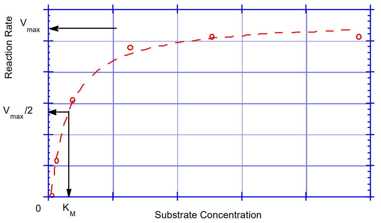
Figure \(\PageIndex{12a}\): Michaelis-Menten plot of enymatic reaction rate vs. [S]

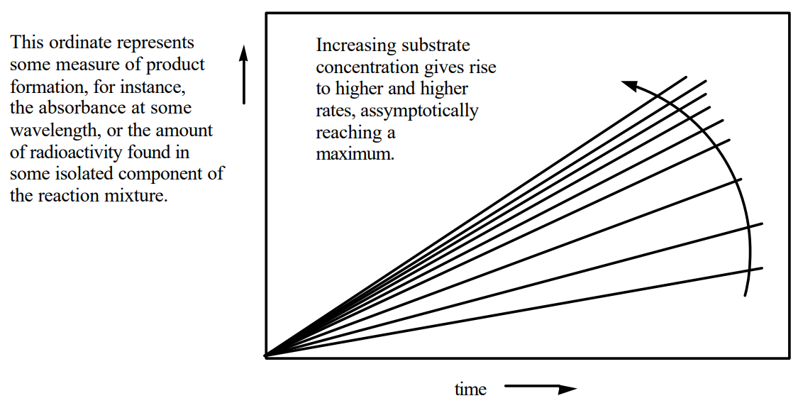
Figure \(\PageIndex{12b}\): Initial reaction rates of product formation vs. time with varying [S]s

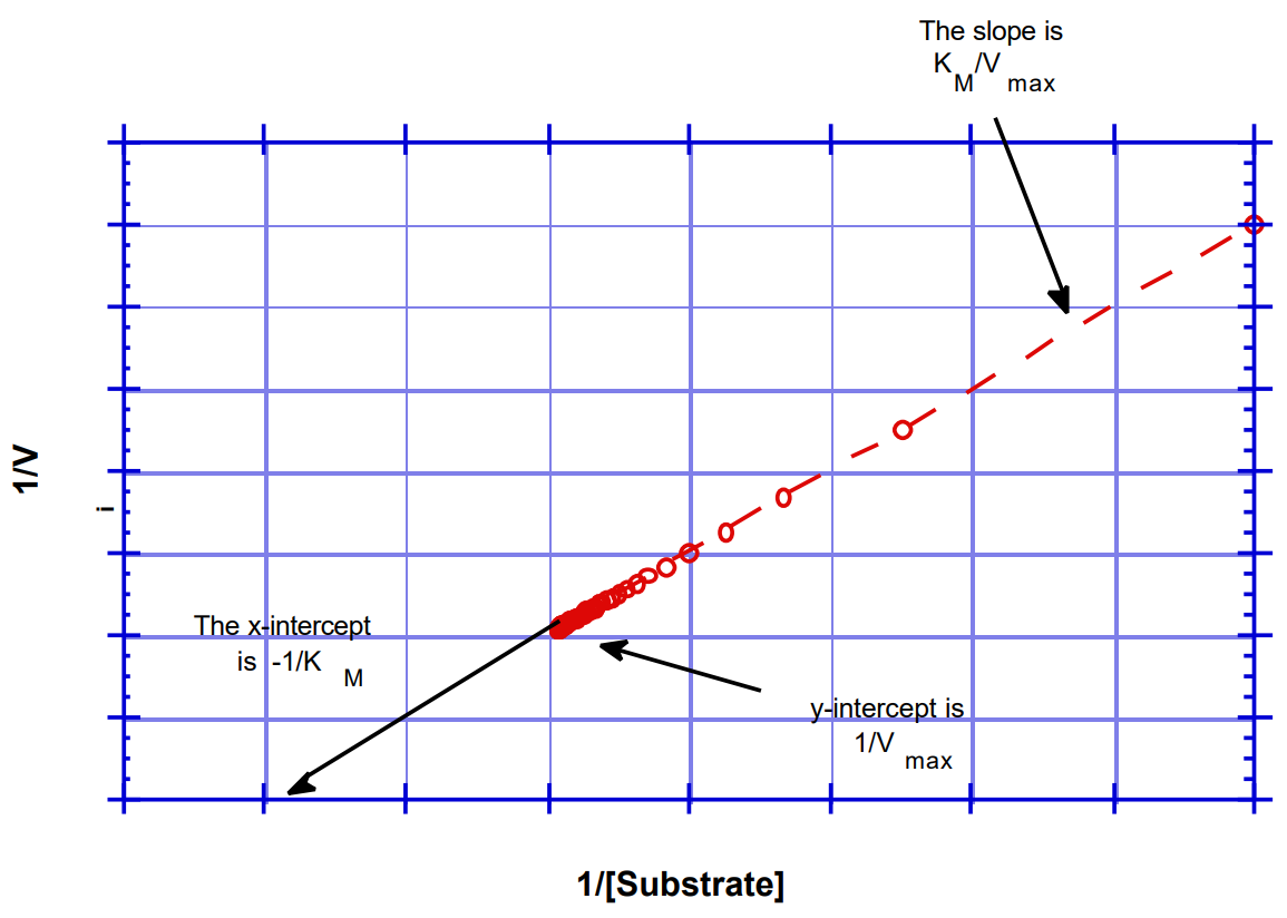
Figure \(\PageIndex{12c}\): Lineweaver-Burk plot

Enzyme Kinetics: Experimental Section.

In this session you will be examining the kinetic properties of PurD or a PurD mutant (G152V) using three different substrates,: glycine, ATP and PRA. You will determine the V_max and K_m for ATP in the presence of saturating levels (8 x Km) of the second and third substrates. Under saturating conditions the complex equation describing the three substrate system, simplifies to the Michaelis Menten Eqn 8 described above. You will be given the concentrations of PRA and glycine to use in your experiments.

B. Kinetic measurements with wild-type and a mutantPurD

The Varian Cary 100 spectrophotometer that you will be using for these experiments can measure the rate of decrease or increase of absorbance at any wavelength over time. The sample holder that you will be using can hold up to 6 cuvettes. However, all of your experiments will be carried out by placing the cuvette in only position 1. Using the spectrophotometer, you will obtain the initial velocities of enough samples to generate a Michaelis-Menten plot. The 6 samples will hold solutions of equal enzyme concentration, but of different substrate concentrations which will range between 0.2 and 5 times the K_m of a given substrate. The substrate concentrations analyzed should not be carried out in order of increasing or decreasing concentrations. The 6 different rates of change in A₃₄₀ nm obtained will be multiplied by the appropriate conversion factors, that you will calculate, to provide 6 different initial velocities. This experiment may need to carried out several times in order to obtain reproducible rates. Once you have a ball park number for your Km, you may want to change the concentrations of substrate you use to obtain better fits to the rate equation. The rates obtained from multiple time points can then be used to obtain K_m, V_max, and to determine k_cat. For the wild-type PurD (without a His-tagged tail) previous experiments have yielded the approximate ranges of K_ms for the three substrates: K_mgly = 270 µM, K_mMgATP = 170 µM, K_mPRA = 97 µM. For the His-tagged protein (both wt and G152V) assume a K_m for ATP of 80 µM. This is an arbitrary number that is known to allow you to obtain good kinetics data. This information should be used to select the initial six substrate concentrations that you will use to obtain your own K_m and V_max for ATP with the His-tagged GAR synthetase that you have isolated. Recall that you were told in the introduction that the His-tagged PurD has activity of 50% of the wild type PurD. Kinetics are interactive. You need to make sure, for example, that if you are using a higher substrate concentration than in a previous run that the initial rate is faster. As noted above the mutant PurD has much lower specific activity and therefore more protein is required for your assays.

Materials:

You have previously prepared all of the solutions required for the kinetics experiments.

Buffer 200 mM Tris (pH 8.0, pH adjusted at 25°C), 100 mM KCl, and 12 mM Mg(OAc)2. This solution will be diluted 1:1 in all assay mixtures giving final concentrations of 100 mM Tris, 50 mM KCl and 6 mM Mg(OAc)2

ATP (1 mL of 200 mM ATP)

glycine (1 mL of 150 mM glycine•HCl )

PEP (1 mL of 100 mM PEP )

NADH (1 mL of 10 mM NADH)

LDH and PK

PurD or mutant PurD that you have isolated

Protocol:

Each group will perform a different kinetic experiment with either the wildtype or the mutant PurD. The data from the entire group will then be pooled for the write up of the kinetics section.

Experiment : Determination of the Km for ATP. You will be monitoring your reactions at 340 nm as you have done previously during your purification of PurD. A sample is given for how to set up your experiments minimizing the amount of pipetting that you will have to do. In all cases the final volume is 1 mL which is adjusted by addition of the appropriate amount of water. Because you are making so many additions to your cuvette, it is a good idea to check off each solution as you add it to the cuvette.

Table 2 A sample set of experiments to determine the Km for ATP

cuvette	Complete buffer includes PK, LDH, NADH, PEP, glycine	[PurD or mutant PurD] and volume	[PRA] and volume	[ATP] volume	H2O volume	total volume
1						1 mL
2						1 mL
3						1 mL
4						1 mL
5						1 mL
6						1 mL

C. Spectrophometric measurements of PurD kinetics experiments (See Section II.

Preparation of the 1.0 mL reaction samples for each set of kinetic experiments:

All of your kinetics will be carried out at a constant temperature. We will use 18°C to minimize the rate of decomposition of one of your substrates, PRA. Therefore all of your reaction components need to be preequilibrated at this temperature.

1. Place a cuvette in slot #1 of the sample holder and take a blank reading. The blank should be buffer with no NADH and is not critical since you are only interested in the rate of change in absorbance. The instrument, however, requires a blank as a reference in order to function accurately.
2. For each experiment with a different concentration of substrate (ATP in the sample protocol described above) add the appropriate volume of substrate stock solution and of H₂O to the cuvette. Check off all the ingredients for your reaction mixture (Table 2) to make sure that you have not forgotten to add anything.
3. To minimize the amount of pipetting, make up a stock solution containing the Buffer mix, PEP, PK, LDH, NADH and add saturating levels of the stable fixed substrate(s). Figure out the total volume of this new solution that will be added to the cuvette. Ultimately the final volume in the cuvette will be 1 mL and variable amounts of water are used to ensure that this volume remains constant.
4. Normally one starts the reaction by the addition of a defined amount of enzyme. In a typical assay you will add 1 to 2 ug of enzyme for wt-PurD. You need to make sure that you have added enough enzyme to observe a reasonable change in absorbance as a function of time. You should have a good feel for how much of your enzyme to use in your reaction because of all of the assays that you have carried out during the purification of PurD. Since each group has isolated their own PurD or a mutant PurD and your specific activities might vary, each group will have to determine the quantity of their enzyme to be added to achieve an easily measurable change in absorbance at 340 nm over a several minute period. In the case of wild type PurD you will then add PurD to each of your cuvettes. PRA will be added last to start the reaction as it is chemically unstable.

   Note

   In order to measure initial rates (allowing for the very least amount of product formation before the sample holder is actually placed in the spectrophotometer), it is necessary to work relatively fast once the PRA is added to the cuvette.

   Note

   For those of you that have purified mutant PurDs, it may be that you will observe ATP hydrolysis in the presence of glycine and the absence of any PRA. You will first carry out your kinetic runs in the absence of any PRA, by starting the reaction with enzyme. The reaction should be monitored for about a min. Then, open the sample chamber, remove the cuvette, add the PRA and return the cuvette to the sample chamber. You will then monitor the reaction for the rest of the kinetics run.

5. When ready, quickly add the PRA solution to the cuvette, place a cap or a piece of parafilm over the top of the cuvette and invert the cuvette several times to effect good mixing (try not to spend more than 10 seconds in the mixing). Then place the cuvette in the sample holder in the spectrophotometer, close the lid, click START.
6. When the 5 minute kinetic run is completed, analyze the data as described in Section II.
7. You now have the data to plot 6 data points or more for one Michaelis-Menten plot depending on how many times you have repeated your kinetic analysis. However, recall that you first have to multiply the \(\Delta\)A/min data (from the spectrophotometer) by the conversion factor to convert the experimentally determined value into mmol of product per min. Also be sure to record the amount of enzyme used in all of your experiments.

Fitting the data to the Michaelis-Menten equation:

A Macintosh computer with the program Kaleidagraph is available in the lab, to do curve fitting of the data. Alternatively you can down load this program from the web onto your home computer(www. synergy.com). To use this program, first, type in the values for the substrate concentration and initial velocity in separate columns (in a data window). Then, type Command-K (or Ctrl-K) to name your columns [X, variable substrate and v, respectively]. Then, generate a plot of the data by typing Command-D (from the keyboard), after which you select the data in the substrate concentration column as the x-coordinate and the data in the initial velocity column as the y-coordinate. Then select General under the Curve Fit menu. Place a check in the box next to the y-coordinate description and click on the Define button. Type m1*m0/(m2+m0); m1=0.01; m2=0.1, after which you click on OK. This brings you back to the previous dialog box; click on the OK button in this box as well. This tells the program to fit the plot to the Michaelis-Menten equation where m1=V_max, m2=K_m, and m0=[Substrate]; the initial values of V_max and K_m are set equal to 0.01 and 0.1, respectively. The program then goes through a series of iterations, allowing V_max and K_m to float, until it gets a good fit (i.e. with an R-value close to 1.0). At this point, if the result of the curve-fit is not displayed on your plot, reselect General under the Curve Fit menu and then place a check in the View box. Print out all the information obtained, with an additional copy for your partner.

In addition to obtaining the V_max and K_m parameters via a direct fitting to the Michaelis-Menten equation, you can also try to obtain these numbers from a Lineweaver-Burk plot. This plot can be obtained from the Kaleidagraph program or by calculating the linear regression yourself. A comparison of the differences obtained (depending on the curve-fitting used) will give you an appreciation of the degree of error in the values of these parameters.

Discussion of the Data: Copies of the data from each of the groups will be distributed to every other group.

From the data obtained, answer the following questions. Feel free to make any other additional comments from the information that has been obtained from these experiments. You will share your data and think about the results on the mutant and wild-type PurDs together.

1. Which PurD, wild-type or mutant, has the largest V_max and what are the relative K_ms for ATP for each PurD?
2. Provide a chemical explanation for your observation that mutant protein shows consumption of NADH (ATP is consumed) in the absence of PRA?

 

Session 7 Instructions for Looking at PurD using RasMol

The protein structures are located at http://biochemistry.lms.mit.edu/1gso.subs.pdb or 1GSO.pdb or 1IOV.pdb. When the structure appears, right click and save the file on your computer. You will learn how to look at the structure of PurD determined crystallographically and of a closely related family member DDL. An understanding of the structures of these two proteins should help you arrive at a reasonable explanation for the kinetic data obtained in the previous sections.

Within Netscape go to Yahoo and enter RasMol. Click on the first entry describing RasMol. This site is linked to two additional sites that you will find helpful. Initially you should click on Tutorial and go to the site from the U. of Southern Maine. This site leads you step by step through the use of RasMol and describes many of the commands that you will need to know. The second site that is also very helpful, especially as you become more sophisticated in the use of RasMol, is called RasMol Reference Manual. This site has been prepared by Roger Sayle, the developer of this program. You might want to bookmark these two sites.

Rasmol is also available on ATHENA

Type “add rasmol” to add the locker

Type “rasmol” or “rasmol filename.pdb” to start the program

Open Rasmac 2.6-ubc or to the version of RasMol you have downloaded.

File:open Go to http://biochemistry.lms.mit.edu/1GSO.pdb (this is the PurD structure) or open 1IOV.pdb (this is the D-ala-D-ala ligase (DDL) structure with a tight binding phosphinate inhibitor bound in the active site) or 1GSO.subs.pdb (this is the structure of PurD in which we have modeled in ADP from the DDL structure and GAR from the structure of GAR transformylase (PurN, Figure 2) . You will familiarize yourself with the structure of PurD and the liganded DDL. You want to convince yourselves that these proteins are structurally homologous and members of the ATP grasp superfamily. Initially you will use the Pull-down menu (File, Edit, Display, Colours, Options etc) on the top of your screen. Look under each heading and familiarize yourself with the transformations that are accessible from this menu. Under Windows: command-line, a second window will open that is white with a RasMol> prompt. Use of this command-line window and commands described below will be essential for allowing you to look at various parts of the PurD and DDL structures.

Display:cartoons Cartoon displays sheet strands as arrows pointing toward the C terminal end of the chain. Note you can not get any information by clicking on the structure, about individual amino acid residues in this display mode.

Colours:structures These commands display your protein with a helices (pink) and b-sheets (yellow). Turns will be in blue if they have been defined by the PDB header. Initially you want to become familiar with the commands that allow you to move your molecule.

1. To rotate the molecule, place the pointer anywhere in the main screen, hold down the mouse button and move the mouse. Dragging up and down rotates the model around the horizontal axis (X) through the molecules center. Dragging left and right rotates around the verticle Y axis. Hold down shift and command keys while dragging left and right to rotate PurD around the Z axis (perpendicular to the screen). To move PurD translationally, hold option and drag. To zoom, hold down the shift key and drag the pointer down the screen to bring the model closer or up to move it farther away. To return to the original setting go to command-line window Rasmol>reset
2. Initially you will want to familiarize yourselves with the domains of these proteins. Pur D is composed of four domains: N, A, B, and C. DDL contains only three domains: N, A, and B. For PurD the N domain includes residues 1-114, the B domain includes residues 122-188, the A domain includes 223-321 and the C domain includes residues 330-425. For DDL the N domain includes residues 1 - 109 , the B domain includes 110 - 184 , the A domain includes residues 185 - 306. You will look at each domain separately using the commands described below and make a plumbing diagram of each domain (see below for an example) and compare the results from each protein. The plumbing diagram should indicate not only the secondary structural features, but also the tertiary features, the spacial relationship of the secondary features to one another. The following commands within the command-line window will be used so that you can look at each domain.

Picking and Selecting:

To select residues in the B domain

Rasmol>restrict 122-188

Restrict selects all atoms specified and hides all others. It does not alter the display of the selected atoms.

Display: sticks

Colour: cpk RasMol draws residues 122-188 as a stick model. The cpk command draws the atoms in the appropriate colors: red for oxygen, blue for nitrogen and gray for carbon. If you try to rotate your molecule, it does so around the center of your entire molecule. You may want to center your molecule around a specific residue.

Rasmol>center His169

You can center this domain around any amino acid or specific atom that you like. If for example you want to center around the a carbon (CA) of His 169

Rasmol>center His169.ca RasMol is picky about the syntax of expressions. If you have trouble go to the manual.

To draw your plumbing diagrams, repeat the above exercise with each domain and each protein. In presenting your diagram think about the tertiary as well as the secondary structure.

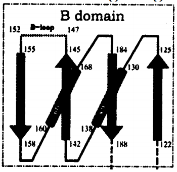
Figure \(\PageIndex{13}\): An example of a Plumbing Diagram: B domain PurD

3. Exploring: You have already been exposed to the restrict command. The select command is equally important.. 
   1. Rasmol> select <return> You have now returned to your entire molecule. Alternatively you can select only certain residues 122-156 etc.
   2. Rasmol > reset <return> Display: sticks Returns full backbone to the screen and centers the rotation to the entire molecule and original orientation.
4. We will use DDL as a representative of the active site of an ATP grasp superfamily protein. This enzyme was crystallized in the presence of ATP and a substrate analog, a phosphinate analog of D-alanine-D-alanine (DD). From your plumbing diagrams above, you should have convinced yourself that this protein is structurally homologous to PurD, especially in the region of ATP. In addition, highlight the B loop residues 140-157, the omega loop residues 208 - 224, and the J loop residues 266-285. These residues should engulf the active site.
   1. Rasmol> select 140-157 
   2. Display: ball and stick
   3. Rasmol> select 208 to 224 
   4. Display: stick
   5. Rasmol> select 266-285 <return>
   6. Display: ball and stick
   7. This process should immediately show you the active site and the loops responsible for its sequestration. DDL has ligands (non-protein and non-water) bound in the active site. We can use these ligands to practice some new commands within Rasmol, but also as a model for how ATP might bind in the active site of PurD. First we will identify the ligands bound in the active site. You will have some surprises.
   8. Open 10V. pdb in Rasmol
   9. Colour: cpk
   10. Rasmol>select hetero and not hoh
   11. Display: ball and stick

Zoom in on the ligands in the ball and stick format. Draw what you see and explain why this observation is unusual given the crystallization conditions. Click on each molecule and the name of the atom in the molecule will appear in the command window. Write down the names of the molecules for future reference. Note that the ball and stick format displays three green balls, two in the active site. These are magnesium ions and are only detectable in this display mode.

Now you will look in the region around the active site in order to identify the amino acid residues that are responsible for binding the substrates. Rasmol> restrict within (10.0, ____) <return>

The 10.0 refers to the number of angstroms around the active site residue or center of interest. Note you must have a decimal point or the command won't work. The ____ refers to molecules you have just identified as being the center of interest. You have written down the names of each substrate and this name should be inserted in place of ___. You can restrict around either of the molecules or specific atoms within these molecules in the active site. You can also select the B, omega and J loops in addition to the small molecules and you should see how the loops surround the active site.

5. Distances: In order for you to know whether an interaction is interesting you must know the distance between the atom of interest in your small molecule and the protein.
   1. Rasmol>restrict within (10.0, ADP) <return>
   2. Display: wireframe
   3. Rasmol>center ADP <return>
   4. Rasmol>set picking monitors <return>
   5. Click on the two atoms of interest, one on your small molecule and one on the protein and a dotted line should appear with the distance indicated. To remove the distances so that new distances can be examined:
   6. Rasmol> set picking ident <return>
   7. Rasmol> monitors off <return>

Questions:

 The adenine nucleotide binds between which two domains in DDL? How are the charges on the phosphates of adenine nucleotide neutralized? What residue(s) plays a key role in binding the 2' and 3' hydroxyl groups of the ribose of the adenine nucleotide? How are the metals bound? Look at the distances between the metals and the ligands to the proteins to convince yourself that the side chains you have chosen are in fact within bonding distance. Determine the distance to the amino acid side chain thought to interact with the 2' and 3' hydroxyls of the ribose. What are the specific interactions that govern adenine binding?

This final exercise should give you a feeling for the nucleotide binding site which is thought to be similar, although not identical, in all ATP grasp superfamily members. Examination of this structure will thus help you to look at the structure of PurD with ATP and GAR placed into the active site of the enzyme by modeling. 1GSO.subs.pdb is a model!!! Nothing has been done to make sure there are no steric clashes between the ATP and GAR added to the PurD structure which was solved in the absence of any ligands. The ATP site was placed into PurD using the premise that this site will be similar to that observed crystallographically in DDL. The GAR site was generated using the structural information from GAR transformylase solved with GAR bound (see Figure 1 with the purine biosynthetic pathway). The binding domain of GAR in the transformylase is a Rossmann fold (\(\alpha\beta\alpha\) structure) and is very similar to the N domain of PurD. Note that the phosphate of GAR is bound to a "P loop", a loop between the N-terminal strand and the first helix.

You will look at this modeled structure in the same fashion that you have looked at empty PurD and DDL with ligands. Draw a picture of the ATP binding site and show, with distances, the residues from PurD that might be involved in binding.

The following instructions might help you to achieve this goal. Clustal W alignments have been made of enzymes involved in the ATP grasp superfamily. The following ligands have been proposed to be important in ATP/ADP binding:

adenine: V143, I285, E187, E188, F189, L190, M275, V155

ribose: E194, K216

\(\alpha\)-P: K145 and Mg

b-P: K105 and both Mgs

Mg: E286 and an \(\alpha\) and \(\beta\) oxygen of phosphates

Mg: N288 and the \(\beta\)-oxygen of P

Rasmol> restrict 143, 285, 187, 188, 190, 275, 155, 194, 216, 145, 105 <return>

Display: Ball & stick

Rasmol> select hetero and not hoh

Display: ball and stick

Rasmol> set picking monitors

Click on any two atoms of interest to display the distance on the screen.

In order to interpret the kinetic results from the entire class, you would like to identify the location of the mutation relative to the ATP/ADP binding site. This structural insight might help you to interpret your results. The following sequence of commands will help you see the location of the mutation.

Pull up and open 1gso.subs.pdb

Rasmol> select 122-188 <return>

Display: backbone

The B domain should be apparent.

Rasmol> select 146-153 <return>

You notice that most of the residues are missing and there is a break in the polypeptide chain. Why?

Rasmol> select hetero and not hoh <return>

Display: ball and stick

Now think about the mutations that you have made at position 152 of the sequence. The corresponding B loop in DDL is residues 140-157. Display these resdiues This display may give you insight about the observed phenotypes of the mutants in PurD.

6. .Saving your work: Scripts
   1. At any time during Rasmol, you can write a script that Rasmol can use to recover your current view. You will want a copy of your active site in your final lab report as a prompt for discussing your kinetic results. The following are instructions as to how to write the Script. Fill the screen with the figure that you wish to preserve. Rasmol > write script CDRs.spt <return> After a brief pause, Rasmol writes the Script. This new file will appear in the same location as the Rasmol program icon. Its icon is a little scroll. The file ending .spt (for script) helps distinguish a script from a coordinate file which ends in pdb or ent.