
9.7: Theories of Reaction Rates
- Page ID
- 41347
\( \newcommand{\vecs}[1]{\overset { \scriptstyle \rightharpoonup} {\mathbf{#1}} } \)
\( \newcommand{\vecd}[1]{\overset{-\!-\!\rightharpoonup}{\vphantom{a}\smash {#1}}} \)
\( \newcommand{\id}{\mathrm{id}}\) \( \newcommand{\Span}{\mathrm{span}}\)
( \newcommand{\kernel}{\mathrm{null}\,}\) \( \newcommand{\range}{\mathrm{range}\,}\)
\( \newcommand{\RealPart}{\mathrm{Re}}\) \( \newcommand{\ImaginaryPart}{\mathrm{Im}}\)
\( \newcommand{\Argument}{\mathrm{Arg}}\) \( \newcommand{\norm}[1]{\| #1 \|}\)
\( \newcommand{\inner}[2]{\langle #1, #2 \rangle}\)
\( \newcommand{\Span}{\mathrm{span}}\)
\( \newcommand{\id}{\mathrm{id}}\)
\( \newcommand{\Span}{\mathrm{span}}\)
\( \newcommand{\kernel}{\mathrm{null}\,}\)
\( \newcommand{\range}{\mathrm{range}\,}\)
\( \newcommand{\RealPart}{\mathrm{Re}}\)
\( \newcommand{\ImaginaryPart}{\mathrm{Im}}\)
\( \newcommand{\Argument}{\mathrm{Arg}}\)
\( \newcommand{\norm}[1]{\| #1 \|}\)
\( \newcommand{\inner}[2]{\langle #1, #2 \rangle}\)
\( \newcommand{\Span}{\mathrm{span}}\) \( \newcommand{\AA}{\unicode[.8,0]{x212B}}\)
\( \newcommand{\vectorA}[1]{\vec{#1}} % arrow\)
\( \newcommand{\vectorAt}[1]{\vec{\text{#1}}} % arrow\)
\( \newcommand{\vectorB}[1]{\overset { \scriptstyle \rightharpoonup} {\mathbf{#1}} } \)
\( \newcommand{\vectorC}[1]{\textbf{#1}} \)
\( \newcommand{\vectorD}[1]{\overrightarrow{#1}} \)
\( \newcommand{\vectorDt}[1]{\overrightarrow{\text{#1}}} \)
\( \newcommand{\vectE}[1]{\overset{-\!-\!\rightharpoonup}{\vphantom{a}\smash{\mathbf {#1}}}} \)
\( \newcommand{\vecs}[1]{\overset { \scriptstyle \rightharpoonup} {\mathbf{#1}} } \)
\( \newcommand{\vecd}[1]{\overset{-\!-\!\rightharpoonup}{\vphantom{a}\smash {#1}}} \)
\(\newcommand{\avec}{\mathbf a}\) \(\newcommand{\bvec}{\mathbf b}\) \(\newcommand{\cvec}{\mathbf c}\) \(\newcommand{\dvec}{\mathbf d}\) \(\newcommand{\dtil}{\widetilde{\mathbf d}}\) \(\newcommand{\evec}{\mathbf e}\) \(\newcommand{\fvec}{\mathbf f}\) \(\newcommand{\nvec}{\mathbf n}\) \(\newcommand{\pvec}{\mathbf p}\) \(\newcommand{\qvec}{\mathbf q}\) \(\newcommand{\svec}{\mathbf s}\) \(\newcommand{\tvec}{\mathbf t}\) \(\newcommand{\uvec}{\mathbf u}\) \(\newcommand{\vvec}{\mathbf v}\) \(\newcommand{\wvec}{\mathbf w}\) \(\newcommand{\xvec}{\mathbf x}\) \(\newcommand{\yvec}{\mathbf y}\) \(\newcommand{\zvec}{\mathbf z}\) \(\newcommand{\rvec}{\mathbf r}\) \(\newcommand{\mvec}{\mathbf m}\) \(\newcommand{\zerovec}{\mathbf 0}\) \(\newcommand{\onevec}{\mathbf 1}\) \(\newcommand{\real}{\mathbb R}\) \(\newcommand{\twovec}[2]{\left[\begin{array}{r}#1 \\ #2 \end{array}\right]}\) \(\newcommand{\ctwovec}[2]{\left[\begin{array}{c}#1 \\ #2 \end{array}\right]}\) \(\newcommand{\threevec}[3]{\left[\begin{array}{r}#1 \\ #2 \\ #3 \end{array}\right]}\) \(\newcommand{\cthreevec}[3]{\left[\begin{array}{c}#1 \\ #2 \\ #3 \end{array}\right]}\) \(\newcommand{\fourvec}[4]{\left[\begin{array}{r}#1 \\ #2 \\ #3 \\ #4 \end{array}\right]}\) \(\newcommand{\cfourvec}[4]{\left[\begin{array}{c}#1 \\ #2 \\ #3 \\ #4 \end{array}\right]}\) \(\newcommand{\fivevec}[5]{\left[\begin{array}{r}#1 \\ #2 \\ #3 \\ #4 \\ #5 \\ \end{array}\right]}\) \(\newcommand{\cfivevec}[5]{\left[\begin{array}{c}#1 \\ #2 \\ #3 \\ #4 \\ #5 \\ \end{array}\right]}\) \(\newcommand{\mattwo}[4]{\left[\begin{array}{rr}#1 \amp #2 \\ #3 \amp #4 \\ \end{array}\right]}\) \(\newcommand{\laspan}[1]{\text{Span}\{#1\}}\) \(\newcommand{\bcal}{\cal B}\) \(\newcommand{\ccal}{\cal C}\) \(\newcommand{\scal}{\cal S}\) \(\newcommand{\wcal}{\cal W}\) \(\newcommand{\ecal}{\cal E}\) \(\newcommand{\coords}[2]{\left\{#1\right\}_{#2}}\) \(\newcommand{\gray}[1]{\color{gray}{#1}}\) \(\newcommand{\lgray}[1]{\color{lightgray}{#1}}\) \(\newcommand{\rank}{\operatorname{rank}}\) \(\newcommand{\row}{\text{Row}}\) \(\newcommand{\col}{\text{Col}}\) \(\renewcommand{\row}{\text{Row}}\) \(\newcommand{\nul}{\text{Nul}}\) \(\newcommand{\var}{\text{Var}}\) \(\newcommand{\corr}{\text{corr}}\) \(\newcommand{\len}[1]{\left|#1\right|}\) \(\newcommand{\bbar}{\overline{\bvec}}\) \(\newcommand{\bhat}{\widehat{\bvec}}\) \(\newcommand{\bperp}{\bvec^\perp}\) \(\newcommand{\xhat}{\widehat{\xvec}}\) \(\newcommand{\vhat}{\widehat{\vvec}}\) \(\newcommand{\uhat}{\widehat{\uvec}}\) \(\newcommand{\what}{\widehat{\wvec}}\) \(\newcommand{\Sighat}{\widehat{\Sigma}}\) \(\newcommand{\lt}{<}\) \(\newcommand{\gt}{>}\) \(\newcommand{\amp}{&}\) \(\definecolor{fillinmathshade}{gray}{0.9}\)The macroscopic discussion of kinetics discussed in previous sections can be now expanded into a more microscopic picture in terms of molecular level properties (e..g, mass and velocities) involving two important theories: (1) collision theory and (2) transition-state theory.
Collision Theory
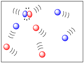
If two molecules need to collide in order for a reaction to take place, then factors that influence the ease of collisions will be important. The more energy there is available to the molecules, the faster they will move around, and the more likely they are to bump into each other. Higher temperatures ought to lead to more collisions and a greater frequency of reactions between molecules. In the drawing below, the cold, sluggish molecules on the left are not likely to collide, but the energetic molecules on the right are due to collide at any time.
The rate at which molecules collide which is the frequency of collisions is called the collision frequency, \(Z\), which has units of collisions per unit of time. Given a container of molecules \(A\) and \(B\), the collision frequency between \(A\) and \(B\) is defined by:
\[Z=N_{A}N_{B}\sigma_{AB}\sqrt{\dfrac{8k_{B}T}{\pi\mu_{AB}}}\]
where:
- NA and NB are the numbers of molecules A and B, and is directly related to the concentrations of A and B.
- The mean speed of molecules obtained from the Maxwell-Boltzmann distribution for thermalized gases
\[ \sqrt{\dfrac{8k_{B}T}{\pi\mu_{AB}}} \]
- \(\sigma_{AB}\) is the averaged sum of the collision cross-sections of molecules A and B. The collision cross section represents the collision region presented by one molecule to another.
- \(\mu\) is the reduced mass and is given by
\[\mu = \dfrac{m_\text{A} m_\text{B}}{m_\text{A} + m_\text{B}}\]
The concepts of collision frequency can be applied in the laboratory: (1) The temperature of the environment affects the average speed of molecules. Thus, reactions are heated to increase the reaction rate. (2) The initial concentration of reactants is directly proportional to the collision frequency; increasing the initial concentration will speed up the reaction.
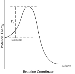
For a successful collision to occur, the reactant molecules must collide with enough kinetic energy to break original bonds and form new bonds to become the product molecules. This energy is called the activation energy for the reaction; it is also often referred to as the energy barrier.
The fraction of collisions with enough energy to overcome the activation barrier is given by:
\[f = e^{\frac{-E_a}{RT}}\]
where:
- \(f\) is the fraction of collisions with enough energy to react
- \(E_a\) is the activation energy
The fraction of successful collisions is directly proportional to the temperature and inversely proportional to the activation energy.
The fraction of successful collisions is directly proportional to the temperature and inversely proportional to the activation energy.
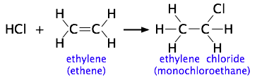
The more complicated the structures of the reactants, the more likely that the value of the rate constant will depend on the trajectories at which the reactants approach each other. This kind of electrophilic addition reaction is well-known to all students of organic chemistry. Consider the addition of a hydrogen halide such as HCl to the double bond of an alkene, converting it to a chloroalkane.
Experiments have shown that the reaction only takes place when the HCl molecule approaches the alkene with its hydrogen-end, and in a direction that is approximately perpendicular to the double bond, as shown at  below.
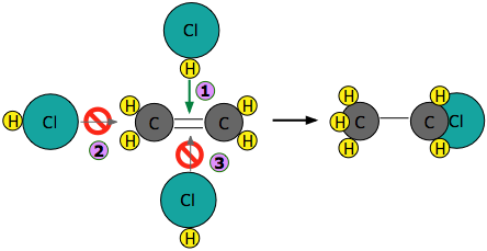
The reason for this becomes apparent when we recall that HCl is highly polar owing to the high electronegativity of chlorine, so that the hydrogen end of the molecule is slightly positive. The steric factor, \(\rho\) is then introduced to represent is the probability of the reactant molecules colliding with the right orientation and positioning to achieve a product with the desirable geometry and stereospecificity. Values of \(\rho\) are generally very difficult to assess and range from 0 to 1, but are sometime estimated by comparing the observed rate constant with the one in which the preexponential constant \(A\) is assumed to be the same as \(Z\).
The lesson you should take from this example is that once you start combining a variety of chemical principles, you gradually develop what might be called "chemical intuition" which you can apply to a wide variety of problems. This is far more important than memorizing specific examples.
All Three Factors Combined
The rate constant of the gas-phase reaction is proportional to the product of the collision frequency and the fraction of successful reactions. As stated above, sufficient kinetic energy is required for a successful reaction; however, they must also collide properly. Compare the following equation to the Arrhenius equation:
\[ k = Z\rho{e^{\frac{-E_a}{RT}}}\]
where
- k is the rate constant for the reaction
- ρ is the steric factor.
- Zρ is the pre-exponential factor, A, of the Arrhenius equation. It is the frequency of total collisions that collide with the right orientation. In practice, it is the pre-exponential factor that is directly determined by experiment and then used to calculate the steric factor.
- Ea is activation energy
- T is absolute temperature
- R is gas constant.
Although the collision theory deals with gas-phase reactions, its concepts can also be applied to reactions that take place in solvents; however, the properties of the solvents (for example: solvent cage) will affect the rate of reactions. Ultimately, collision theory illustrates how reactions occur; it can be used to approximate the rate constants of reactions, and its concepts can be directly applied in the laboratory. Read this for a more detailed discussion of Collision Theory.
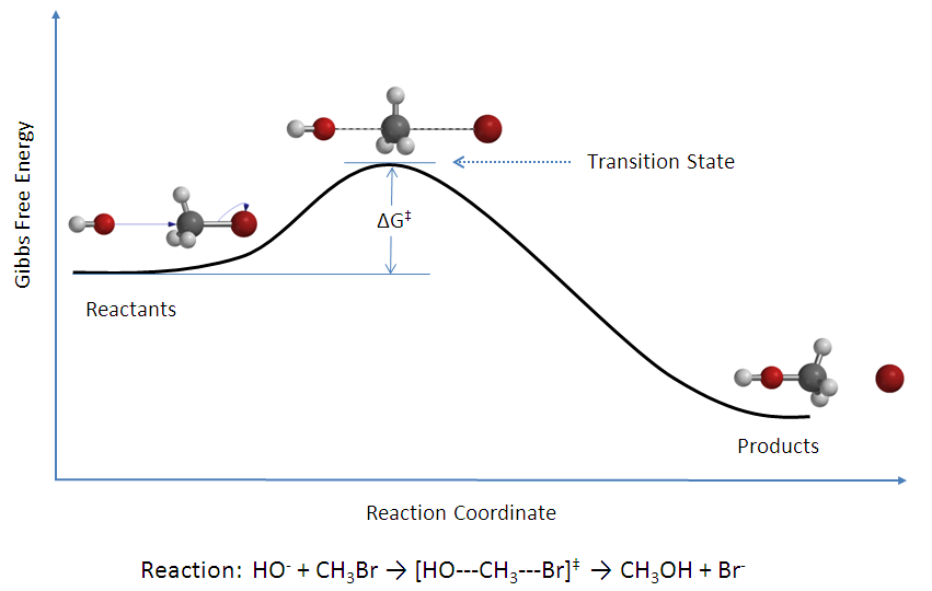
Transition-State Theory
Transition state theory (TST) provides a more accurate alternative to the previously used Arrhenius equation and the collision theory. The transition state theory attempts to provide a greater understanding of activation energy, \(E_a\), and the thermodynamic properties involving the transition state. Collision theory of reaction rate, although intuitive, lacks an accurate method to predict the probability factor for the reaction. The theory assumes that reactants are hard spheres rather than molecules with specific structures. In 1935, Henry Eyring helped develop a new theory called the transition state theory to provide a more accurate alternative to the previously used Arrhenius equation and the collision theory. The Eyring equation involves the statistical frequency factory, v, which is fundamental to the theory.
According to TST, between the state where molecules are reactants and the state where molecules are products, there is a state known as the transition state. In the transition state, the reactants are combined in a species called the activated complex. The theory suggests that there are three major factors that determine whether a reaction will occur:
- The concentration of the activated complex
- The rate at which the activated complex breaks apart
- The way in which the activated complex breaks apart: whether it breaks apart to reform the reactants or whether it breaks apart to form a new complex, the products.
Collision theory proposes that not all reactants that combine undergo a reaction. However, assuming the stipulations of the collision theory are met and a successful collision occurs between the molecules, transition state theory allows one of two outcomes: a return to the reactants, or a rearranging of bonds to form the products.
Consider a bimolecular reaction:
\[A~+B~\rightarrow~C \label{2}\]
\[K = \dfrac{[C]}{[A][B]} \label{3}\]
where \(K\) is the equilibrium constant. In the transition state model, the activated complex AB is formed:
\[A~+~B~\rightleftharpoons ~AB^\ddagger~\rightarrow ~C \label{4}\]
\[K^\ddagger=\dfrac{[AB]^\ddagger}{[A][B]} \label{5}\]
There is an energy barrier, called activation energy, in the reaction pathway. A certain amount of energy is required for the reaction to occur. The transition state, \(AB^\ddagger\), is formed at maximum energy. This high-energy complex represents an unstable intermediate. Once the energy barrier is overcome, the reaction is able to proceed and product formation occurs.
The rate of a reaction is equal to the number of activated complexes decomposing to form products. Hence, it is the concentration of the high-energy complex multiplied by the frequency of it surmounting the barrier.
\[\begin{eqnarray} rate~&=&~v[AB^\ddagger] \label{6} \\ &=&~v[A][B]K^\ddagger \label{7} \end{eqnarray} \]
The rate can be rewritten:
\[rate~=~k[A][B] \label{8}\]
Combining Equations \(\ref{8}\) and \(\ref{7}\) gives:
\[ \begin{eqnarray} k[A][B]~&=&~v[A][B]K^\ddagger \label{9} \\ k~&=&~vK^\ddagger \label{10} \end{eqnarray} \]
where
- \(v\) is the frequency of vibration,
- \(k\) is the rate constant and
- \(K ^\ddagger \) is the thermodynamic equilibrium constant.
Statistical mechanics (not shown) provides that the frequency, v, is equivalent to the thermal energy, kBT, divided by Planck's constant, h.
\[v~=~\dfrac{k_BT}{h} \label{11}\]
where
- \(k_B\) is the Boltzmann's constant (1.381 x 10⁻²³ J/K),
- \(T\) is the absolute temperature in Kelvin (K) and
- \(h\) is Planck's constant (6.626 x 10⁻³⁴ Js).
Substituting Equation \(\ref{11}\) into Equation \(\ref{10}\) :
\[k~=~\dfrac{k_BT}{h}K^\ddagger \label{12}\]
Equation \({ref}\) is often tagged with another term \((M^{1-m})\) that makes the units equal with \(M\) is the molarity and \(m\) is the molecularly of the reaction.
\[k~=~\dfrac{k_BT}{h}K^\ddagger (M^{1-m}) \label{E12}\]
It is important to note here that the equilibrium constant \(K^\ddagger \) can be calculated by absolute, fundamental properties such as bond length, atomic mass, and vibration frequency. This gives the transition rate theory the alternative name absolute rate theory, because the rate constant, k, can be calculated from fundamental properties.
Thermodynamics of Transition State Theory
To reveal the thermodynamics of the theory, \(K^\ddagger\) must be expressed in terms of \(\Delta {G^{\ddagger}}\). \(\Delta {G^{\ddagger}}\) is simply,
\[\Delta{G}^{o\ddagger} = G^o (transitionstate) - G^o (reactants)\]
By definition, at equilibrium, \(\Delta {G^{\ddagger}}\) can be expressed as:
\[\Delta {G^{\ddagger}} = -RT \ln K^{\ddagger}\]
Rearrangement gives:
\[[K]^\ddagger = e^{ -\frac{\Delta{G}^\ddagger}{RT} }\]
From Equation \(\ref{E12}\)
\[ \color{red} k = ve^{ -\frac{\Delta{G}^{\ddagger}}{RT}} (M^{1-m})\]
It is also possible to obtain terms for the change in enthalpy and entropy for the transition state. Because
\[\Delta{G^\ddagger} = \Delta{H^\ddagger} - T\Delta{S^\ddagger}\]
it follows that the derived equation becomes,
\[k = \dfrac{k_BT}{h} e^{\Delta{S}^\ddagger /R} e^{-\Delta H^\ddagger/RT} M^{1-m} \label{Eyring}\]
Equation \(\ref{Eyring}\) is known as the Eyring Equation and was developed by Henry Eyring in 1935, is based on transition state theory and is used to describe the relationship between reaction rate and temperature. It is similar to the Arrhenius Equation, which also describes the temperature dependence of reaction rates.
The linear form of the Eyring Equation is given below:
\[\ln{\dfrac{k}{T}}~=~\dfrac{-\Delta H^\dagger}{R}\dfrac{1}{T}~+~\ln{\dfrac{k_B}{h}}~+~\dfrac{\Delta S^\ddagger}{R} \label{17}\]
The values for \(\Delta H^\ddagger\) and \(\Delta S^\ddagger\) can be determined from kinetic data obtained from a \(\ln{\dfrac{k}{T}}\) vs. \(\dfrac{1}{T}\) plot. The Equation is a straight line with negative slope, \(\dfrac{-\Delta H^\ddagger}{R}\), and a y-intercept, \(\dfrac{\Delta S^\ddagger}{R}+\ln{\dfrac{k_B}{h}}\).
Conclusion
In this article, the complete thermodynamic formulation of the transition state theory was derived. This equation is more reliable than either the Arrhenius equation and the equation for the Collision Theory. However, it has its limitations, especially when considering the concepts of quantum mechanics. Quantum mechanics implies that tunneling can occur, such that particles can bypass the energy barrier created by the transition state. This can especially occur with low activation energies, because the probability of tunneling increases when the barrier height is lowered.
In addition, transition state theory assumes that an equilibrium exists between the reactants and the transition state phase. However, in solution non-equilibrium situations can arise, upsetting the theory. Several more complex theories have been presented to correct for these and other discrepancies. This theory still remains largely useful in calculating the thermodynamic properties of the transition state from the overall reaction rate. This presents immense usefulness in medicinal chemistry, in which the study of transition state analogs is widely implemented.
References
- Chang, Raymond. Physical Chemistry for the Biosciences. University Science Books, California 2005
- Truhlar, D. G.; Garrett, B. C.; Klippenstein, S. J., Current Status of Transition-State Theory. The Journal of physical chemistry 1996, 100, (31), 12771-12800
- Laidler, K.; King, C., Development of transition-state theory. The Journal of physical chemistry 1983, 87, (15), 2657
- Lienhard, Gustav, Enzyme Catalysis and Transition -State Theory: Transition State Analogs. Cold Spring Harb Symp Quant Biol 1972. 36:45-51
Contributors and Attributions
- Phong Dao, Bilal Latif, Lu Zhao (UC Davis)