1.3: Quantum Numbers

Quantum Numbers

The wave equations used to describe the electron configuration require at least 3 variables called quantum numbers. Changing the quantum numbers, the variables in the wave equation, changes the energy of the electron. Each electron has its own unique set of quantum numbers. The shapes shown for the quantum orbital are created by graphing the wave equations in three dimensions. The outer boundary of the shape is the cut-off point for the location of the electron 90% of the time. Since the electron in an orbital travels randomly both in direction and speed, pinpointing its location or path is impossible (this is the famous Heisenberg uncertainty principle: “The more precisely the position is determined, the less precisely the momentum is known in this instant, and vice versa.”). Thus an orbital represents the “container” where an electron is probably located, and each orbital is a graph of the wave equation for a specific energy.

The First Quantum Number: Energy level or shell, n

The first quantum number describes the radius the electron exists away from the nucleus. So n = 1 means that the electrons with this quantum number will be closest to the nucleus. n = 2 will be in the second layer, n = 3 will be in the third layer, and so on up to n = 7.

The Second Quantum Number: Orbital Shape subshell, \(\ell\)

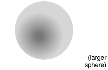
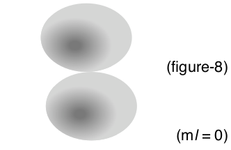
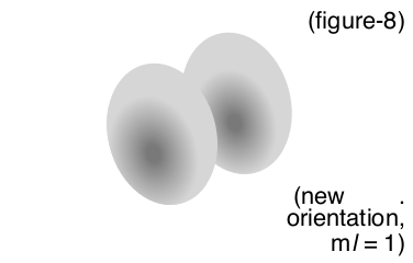
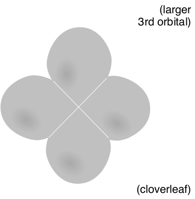
The second quantum number determines the shape of the orbital, which is the location where electrons can be found in the atom. The number tells you how many nodes are in the shape, where a node is the crossing point in the shape. So \(\ell\) = 0 has no crossing points and will be just a sphere like we expect of an atom (recall the electron location, or electron cloud when all orbitals are combined, is the boundary of the atom). \(\ell\) = 1 has 1 crossing point and looks like a figure-8. \(\ell\) = 2 has 2 crossing points and looks like a four-leaf clover. \(\ell\) = 3 has 3 nodes and is a bit complicated (\(\ell\) = 4 is the highest orbital for this number). The shapes are labeled by either numbers or letters: \(\ell\) = 0 = s; \(\ell\) = 1 = p; \(\ell\) = 2 = d; \(\ell\) = 3 = f.

The Third Quantum Number: Orientation in Three Dimensional Space

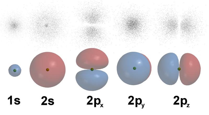
The third quantum number, m l is used to designate orientation in space. The figure-8 shape with \(\ell\) = 1, has three shapes needed to completely fill the spherical shape of an electron cloud. That is combining figure-8 shapes going up and down (z-axis), left and right (x-axis), and back and forth (y-axis), the entire electron cloud will be filled with figure-8 orbitals. It takes three orientations for figure-8 orbital, \(\ell\) = 1, five for the cloverleaf orbital, \(\ell\) = 2, and seven for \(\ell\) = 3 ( \(\ell\) + 1, or consecutive odd numbers).

The 3 p-orbital (s orbital has only one orientation, it changes only its size) (The upper dots represent multiple “snapshots” showing the location of an electron over time.)		http://commons.wikimedia.org/wiki/File:AOs-3D-dots.png
The 5 d-orbital		https://es.wikipedia.org/wiki/Archivo:Orbitalesd.JPG
The 7 f-orbitals		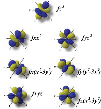https://es.wikipedia.org/wiki/Archivo:F_orbitals.png

The Spin Quantum Number: Only Two Electrons per Orbital

There is a fourth quantum number that doesn’t describe the shape or energy of an electron. This is the spin quantum number, m_s . It turns out that quantum theory requires only two electrons to exist inside any single orbital, where a single orbital has its own size, shape, and orientation. So the two electrons have different spins with 1⁄2 spin (up) and –1⁄2 spin (down). Spin is a property an electron exhibits when it is placed in a magnetic field. Certain values are allowed for the different quantum numbers: n, can be 1 to 7; l, can be (n – 1) to 0 for each energy level n; m\(_{\ell}\) can be -\(\ell\) to 0 to \(\ell\) for each subshell, \(\ell\); and spin is 1⁄2 then – 1⁄2 for every orbital. This means that certain combinations of quantum numbers are not allowed. For example, the following quantum numbers break the rules: (0,0,0,1⁄2) because n ≠ 0; (2,2,-1, 1⁄2) because \(\ell\) must be smaller than n; (3,2,3,1⁄2) because m\(_{\ell}\) is larger than \(\ell\); (3,2,-3,1⁄2) because m\(_{\ell}\)is smaller than -\(\ell\); and (1,0,0, 3⁄4) since m_s must be only 1⁄2 or -1⁄2.

Summary of Quantum Numbers

Variable	n	\(\ell\)	m\(_{\ell}\)	ms
Names of quantum numbers	Principle Quantum Numbers	Angular Momentum Quantum Number	Magnetic Quantum Number	Electron Spin Quantum Number
Possible numbers	n = 1,2,..., 7	\(\ell\)	m\(_{\ell}\) = -\(\ell\),...,0,...,\(\ell\)	\(\frac{1}{2}\) or \(-\frac{1}{2}\)
Also known as	Energy Level or shell	Shape of the Orbital of Subshell, \(\ell\) equals the number of modes or crossing points	Orientation or Alignment along an axis or in a plane	Spin
Physical Representation	Distance from nucleus	s-orbital is a sphere p-orbital is a figure-8 d-orbital is a cloverleaf f-orbitals has 8 & 6 loves	For example, the figure-8 shape may lie on the x, y,&z-axes. d & f-shapes have planes of symmetry.	Arrows up or down for magnetic alignment
Periodic Table Characteristic	Row Number	Periodic table blocks	\(\frac{1}{2}\) of each block is assigned a number line with 0 in the middle	The first half of a block has spin up and the second has spin down

The following examples show how the quantum numbers are translated into three dimensional shapes.

Examples of Quantum Numbers and Shapes

Second Energy Level p-orbital

Description	Quantum Numbers	3d shape
First Energy Orbital, lowest energy	(1, 0, 0, 1/2) n = 1 first energy level \(\ell\) = 0 = s-orbital shape
First Energy Orbital, but for 2^nd electron	(1, 0, 0, –1/2) Same orbital and energy as above. but second electron has opposite spin.
Second Energy Level Orbital	(2, 0, 0, 1/2) n = 2 = second energy level \(\ell\) = 0 = s-orbital
Second Energy Level p-orbital	(2, 1, 0, 1/2) n = 2 = second energy level \(\ell\) = 1 = p-orbital (higher energy than s–orbital)
Second Energy Level p-orbital	(2, 1, 0, 1/2) Same orbital and energy as above, but oriented on a different axis (three possible orientations)
Third Energy Level with d-orbital shape	(3, 2, 0, 1/2) n = 3 = third energy level \(\ell\) = 2 = d-orbital (five possible orientations)

Using the Periodic Table to Determine Quantum Numbers

Quantum numbers are unique to each electron. For example the quantum numbers for the first ten electrons are all different:
1st = {1,0,0,1⁄2} ; 2nd = {1,0,0,–1⁄2}
3rd = {2,0,0,1⁄2} ; 4th = {2,0,0,–1⁄2} ;
5th = {2,1,–1,1⁄2}, 6th = {2,1,0,1⁄2} ; 7th = {2,1,1,1⁄2}
8th = {2,1,–1,–1⁄2}, 9th = {2,1,0,–1⁄2} ; 10th = {2,1,1,–1⁄2}

For every atom these quantum numbers would be used for the first ten electrons, because they represent the lowest ten energies for electrons. Remarkably the periodic table, developed by examining the chemical and physical properties of elements, provides a clear diagram for determining the quantum numbers of electrons. To use the periodic table to determine quantum numbers it must be divided into blocks and the blocks divided in half (and square 2 with He is moved next to square 1 with H.) The row numbers mostly match the principle quantum number, n (d-block and f-block must use n’s one less than the row number and two less than the row number respectively). The blocks match the the angular momentum quantum number, \(\ell\), and both letter and number values are given. m\(_{\ell}\) is shown as a pair of number lines and m_s is positive for the first half of the block and negative for the second half.

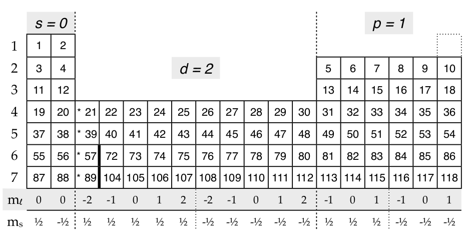
Here’s some examples of quantum numbers of electrons using this divided periodic table:
The 1st electron in any atom has {1,0,0,1⁄2}: row 1, s-block, m l =0, m s =0
The 8th electron in any atom has {2,1,-1,-1⁄2}: row 2, p-block, m l =-1, m s =-1⁄2
The 75th electron in any atom has {5,2,2,1⁄2} : row 6 but for the d-block the n, principle quantum number is one less than the row number, hence the 5, d-block, m l =2, m s =1⁄2
The 84th electron in any atom has {6,1,-1,-1⁄2}: 6th row, p-block, m l =-1, m s =-1⁄2

If we add the f block (with f = 3)

Using the divided periodic table for electrons in the f-block, the 68th electron’s quantum numbers are {4,3,0,-1⁄2}; 6th row but back 2 for the f-block so 4 is used, f-block = 3, m l =0, m s =-1⁄2 And the 94th electron has {5,3,2,1⁄2}.

A common question about quantum numbers might ask, “What is the highest energy electron for the element scandium, Sc?” To answer this question you would find the last electron needed for Sc, which is electron 21, and then use it’s quantum numbers: {3,2,-2,1⁄2}. Just remember that electrons in the d-block have n equal to the row number –1 (row number minus one) and the electrons in the f-block have n equal to the row number –2.

Contributors

• Kenneth Pringle and Curriki. This content is licensed under a Creative Commons Attribution Share-Alike 3.0 License.