Gaussian Integrals

Last updated
Save as PDF

Page ID: 5551

\( \newcommand{\vecs}[1]{\overset { \scriptstyle \rightharpoonup} {\mathbf{#1}} } \) \( \newcommand{\vecd}[1]{\overset{-\!-\!\rightharpoonup}{\vphantom{a}\smash {#1}}} \)\(\newcommand{\id}{\mathrm{id}}\) \( \newcommand{\Span}{\mathrm{span}}\) \( \newcommand{\kernel}{\mathrm{null}\,}\) \( \newcommand{\range}{\mathrm{range}\,}\) \( \newcommand{\RealPart}{\mathrm{Re}}\) \( \newcommand{\ImaginaryPart}{\mathrm{Im}}\) \( \newcommand{\Argument}{\mathrm{Arg}}\) \( \newcommand{\norm}[1]{\| #1 \|}\) \( \newcommand{\inner}[2]{\langle #1, #2 \rangle}\) \( \newcommand{\Span}{\mathrm{span}}\) \(\newcommand{\id}{\mathrm{id}}\) \( \newcommand{\Span}{\mathrm{span}}\) \( \newcommand{\kernel}{\mathrm{null}\,}\) \( \newcommand{\range}{\mathrm{range}\,}\) \( \newcommand{\RealPart}{\mathrm{Re}}\) \( \newcommand{\ImaginaryPart}{\mathrm{Im}}\) \( \newcommand{\Argument}{\mathrm{Arg}}\) \( \newcommand{\norm}[1]{\| #1 \|}\) \( \newcommand{\inner}[2]{\langle #1, #2 \rangle}\) \( \newcommand{\Span}{\mathrm{span}}\)\(\newcommand{\AA}{\unicode[.8,0]{x212B}}\)

The Gaussian function (named after Carl Friedrich Gauss) is a function of the form:

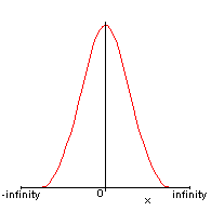
\[e^{-\alpha x^2}\]

and is a characteristic symmetric "bell curve" shape that quickly falls off.

The area under the curve is:

\[I_0(\alpha )=\int_{-\infty}^{\infty}\,e^{-\alpha x^2}\,dx=2\int_{0}^{\infty}\,e^{-\alpha x^2}\,dx\]

The square of \(I_0(a)\) can be written in the form

\[\biggr(I_0(\alpha )\biggr)^2=4\int_{0}^{\infty}dy\int_{0}^{\infty}dz\;e^{-\alpha(y^2+z^2)}\]

Now convert to plane polar coordinates, letting \(r^2 = x^2 + y^2\) and \(dx\; dy = r\;dr\;d\theta\). The appropriate limits of integration over all space in spherical polar coordinates are \(0 < r < \infty\) and \(0 < \theta < \pi/2\) so

\[\biggr(I_0(\alpha )\biggr)^2=4\int_{0}^{\frac{\pi}{2}}d\theta \int_{0}^{\infty}dr\; e^{-\alpha\,r^2}\]

which is elementary and gives

\[\biggr(I_0(\alpha )\biggr)^2=4\frac{\pi }{2}\frac{1}{2\alpha }=\frac{\pi }{\alpha }\]

so that

\[I_0(\alpha) =\sqrt{\frac{\pi }{\alpha }}\]

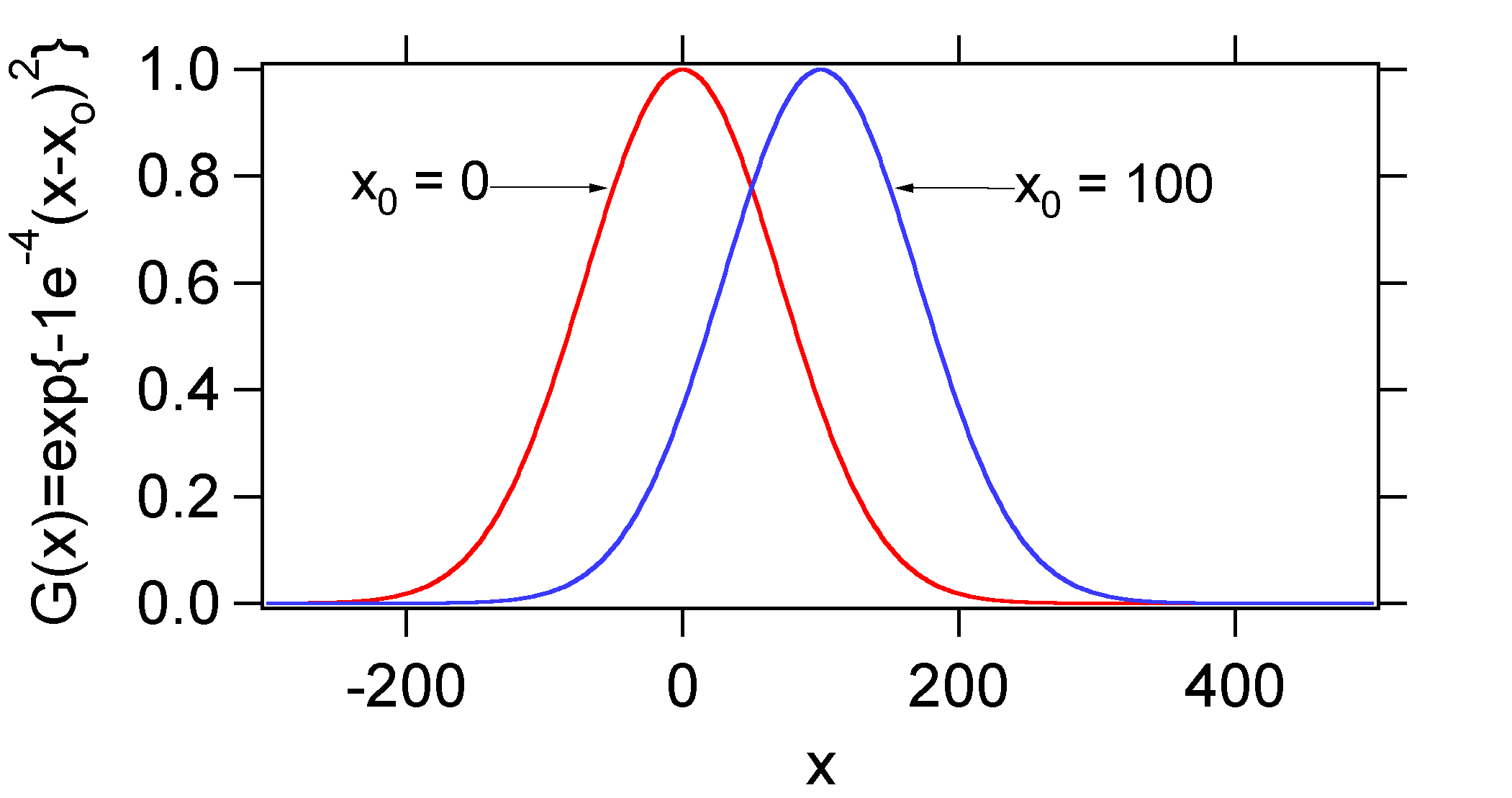
Note that the Gaussian function \(e^{-\alpha x^2}\) is centered at zero. In general, we can express a Gaussian centered at any position \(x_0\) as \(e^{-\alpha(x-x_0)^2}\).

Example 1:
For example, if we let a = 0.0001 we can plot two Gaussian using the above functional form. Notice that if we integrate either one of these the magnitude of the integral is the same. This is evident from inspection since the integral is the area under the curve and the areas are both the same. To see this mathematically, consider the integral \[I_0(\alpha) =\int_{-\infty}^{\infty}\,e^{-\alpha(x-x_0)^2}dx=2\int_{0}^{\infty}\,e^{-\alpha(x-x_0)^2}dx\] We make the substitution \(u = x – x_0\), then \(du = dx\). In that case \[I_0(\alpha) =\int_{-\infty}^{\infty}\,e^{-\alpha\,u^2}du=2\int_{0}^{\infty}e^{-\alpha\,u^2}du\] Which is identical to the integral we started with above.

Example 1:

For example, if we let a = 0.0001 we can plot two Gaussian using the above functional form.

Notice that if we integrate either one of these the magnitude of the integral is the same. This is evident from inspection since the integral is the area under the curve and the areas are both the same. To see this mathematically, consider the integral

\[I_0(\alpha) =\int_{-\infty}^{\infty}\,e^{-\alpha(x-x_0)^2}dx=2\int_{0}^{\infty}\,e^{-\alpha(x-x_0)^2}dx\]

We make the substitution \(u = x – x_0\), then \(du = dx\). In that case

\[I_0(\alpha) =\int_{-\infty}^{\infty}\,e^{-\alpha\,u^2}du=2\int_{0}^{\infty}e^{-\alpha\,u^2}du\]

Which is identical to the integral we started with above.

Note that often Gaussian are written in the form

\[e^{-(x-x_0)^2/2\sigma^2}\]

Integration leads to an area of

\[\int_{-\infty}^{\infty}e^{-(x-x_0)^2/2\sigma^2}dx=\frac{1}{\sqrt{2\pi} \sigma}\]

In this case \(\sigma\) is called the standard deviation. We can also relate \(\sigma\) to the full-width-at-half-maximum (\(\text{FWHM}\)). This is done by recognizing that the magnitude of the function is 1 at its peak. Therefore, we can solve for \(x\) when

\[e^{-(x-x_0)^2/2\sigma^2}=\frac{1}{2}\]

\[x=x_0\pm\sqrt{2\ln2}\sigma\]

and the \(\text{FWHM}\) is

\[\text{FWHM}=2\sqrt{2\ln2}\sigma\]

Contributors

Stefan Franzen (North Carolina State University)