5-8: Harmonic Oscillators in Higher Dimensions

As with 2-D and 3D participle a box problems, is is relatively simple to extend the one dimensional harmonic oscillator to two or the three dimensions.

Two Dimensional Harmonic Oscillator

In more than one dimension, there are several different types of Hooke's law forces that can arise. Consider a diatomic molecule \(AB\) separated by a distance \(r\) with an equilibrium bond length \(r_{eq}\). If we consider the bond between them to be approximately harmonic, then there is a Hooke's law force between then of the form

\[F=-k(r-r_{eq}) \label{5.8.1}\]

which arises from a potential energy

\[V=\dfrac{1}{2}k(r-r_{eq})^2 \label{5.8.2}\]

Note, however, that if the molecule exists in two dimensions (i.e., a nonlinear polyatomic molecule), then \(r=|r|\), where \(\vec{r}\) is the relative vector \(\vec{r}=r_A -r_B =(x,y)\) and \(r=\sqrt{x^2 +y^2}\). The Hooke's law potential is no longer a sum of terms involving only \(x\) and only \(y\). As discussed below, this is also true in three dimensions where \(\vec{r}=(x,y,z)\) and \(r=\sqrt{x^2 +y^2 +z^2}\).

For now, let us take \(r_{eq}=0\) as an approximation. Then, in two dimensions, the Hooke's law potential becomes a harmonic potential in \(x\) and a harmonic potential in \(y\):

\[V(x,y)=\dfrac{1}{2}k(x^2 +y^2) \label{5.8.3}\]

and the classical energy

\[ \underset{\text{kinetic energy}}{\dfrac{p_{x}^{2}}{2\mu}+\dfrac{p_{y}^{2}}{2\mu}} + \underset{\text{potential energy}}{\dfrac{1}{2}k(x^2 +y^2)}=E \label{5.8.4}\]

where \(\mu\) is known as the reduced mass of the diatomic

\[\mu=\dfrac{m_A m_B}{m_A +m_B} \label{5.8.5}\]

Now we see that the classical energy is a sum of terms involving motion and forces in the \(x\) direction and motion and forces in the \(y\) direction:

\[\begin{align*}E &= \varepsilon_x +\varepsilon_y \\ \varepsilon_x &= \dfrac{p_{x}^{2}}{2\mu}+\dfrac{1}{2}kx^2 \\ \varepsilon_y &= \dfrac{p_{y}^{2}}{2\mu}+\dfrac{1}{2}ky^2\end{align*} \label{5.8.6}\]

As with the particle in a two-dimensional box, we will need two independent integers \(n_x\) and \(n_y\) to satisfy the boundary conditions along the \(x\) and \(y\) directions, and the allowed values of \(\varepsilon_x\) and \(\varepsilon_y\) become

\[\varepsilon_{n_x}=\left ( n_x+\dfrac{1}{2} \right )h\nu \;\;\;\; \varepsilon_{n_y}=\left ( n_y +\dfrac{1}{2} \right )h\nu \label{5.8.7}\]

so that the allowed values of the total energy are

\[E_{n_x ,n_y}=(n_x +n_y +1)h\nu \label{5.8.8}\]

Also, as with the particle in a two-dimensional box, the wave functions are products of harmonic oscillator wave functions in the \(x\) and \(y\) directions. Some examples are

\[\begin{align*}\psi_{00} (x,y) &= \left ( \dfrac{\alpha}{\pi} \right )^{1/2}e^{-\alpha (x^2 +y^2)/2}\\ \psi_{10} (x,y) &= \left ( \dfrac{4\alpha^3}{\pi} \right )^{1/4}\left ( \dfrac{\alpha}{\pi} \right )^{1/4} xe^{-\alpha (x^2 +y^2)/2}\\ \psi_{11}(x,y) &= \left ( \dfrac{4\alpha^3}{\pi} \right )^{1/2}xye^{-\alpha (x^2 +y^2)/2}\end{align*} \label{5.8.9}\]

Figure \(\PageIndex{1}\) compares two such wave functions, \(\psi_{00}(x,y)\) and \(\psi_{22}(x,y)\):

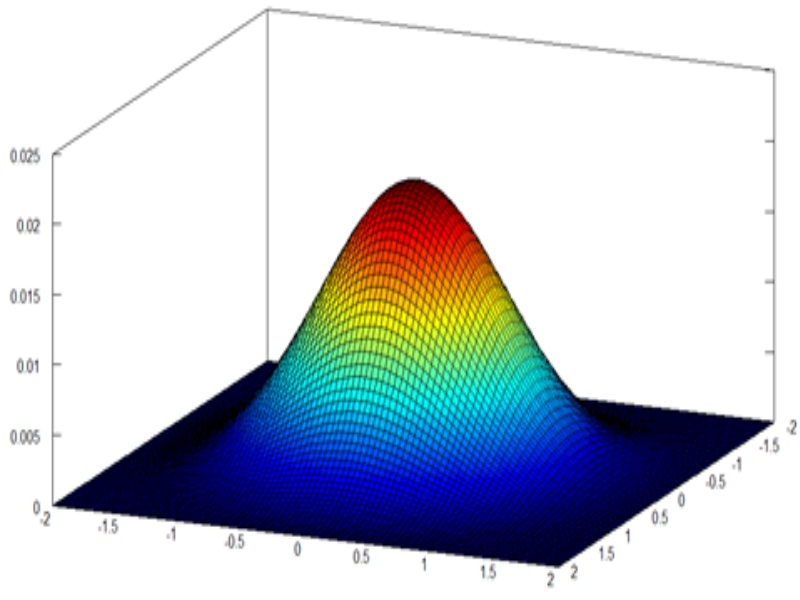
Figure \(\PageIndex{1}\): Wave functions for a symmetric two-dimensional harmonic oscillator. (left) 1st eigenfunction \(\psi_{00}(x,y)\) and (right) 4th eigenfunction \(\psi_{22}(x,y)\). Images used with permission from Wikipedia. Note the nodes in the higher energy eigenstates.

Three Dimensional Harmonic Oscillator

All of this generalizes straightforwardly to three dimensions, again assuming \(r_{eq}=0\). In this case

\[V(x,y,z)=\dfrac{1}{2}k(x^2 +y^2 +z^2) \label{5.8.10}\]

the classical energy is

\[\dfrac{p_{x}^{2}}{2\mu}+\dfrac{p_{y}^{2}}{2\mu}+\dfrac{p_{z}^{2}}{2\mu}+\dfrac{1}{2}k(x^2 +y^2 +z^2)=E \label{5.8.11}\]

which is a sum of three terms \(\varepsilon_x +\varepsilon_y +\varepsilon_z\), and we need three integers \(n_x\), \(n_y\), and \(n_z\). The allowed values of these three energies will be

\[\varepsilon_{n_x}=\left ( n_x +\dfrac{1}{2} \right ) h\nu \;\;\;\; \varepsilon_{n_y}=\left ( n_y +\dfrac{1}{2} \right )h\nu \;\;\;\; \varepsilon_{n_z}=\left ( n_z +\dfrac{1}{2} \right ) h\nu\label{5.8.12}\]

and the allowed values of the total energy will be

\[E_{n_x n_y n_z}=\left ( n_x +n_y +n_z +\dfrac{3}{2} \right )h\nu\label{5.8.13}\]

Similarly, the wave functions will be products of one-dimensional harmonic oscillator functions in the \(x\), \(y\), and \(z\) directions. Thus, the ground state would be

\[\psi_{000}(x,y,z)=\left ( \dfrac{\alpha}{\pi} \right )^{3/4}e^{-\alpha (x^2 +y^2 +z^2)/2}\label{5.8.14}\]

and other wave functions can be constructed in a similar manner. For example, the lowest energy state of the three dimensional harmonic oscillator (via Equation \(\ref{5.8.13}\)), the zero point energy, is

\[E_{n_x=0, n_y=0, n_z=0} = \dfrac{3}{2} h \nu \label{5.8.15}\]

Obviously, the higher energy states are very degenerate—many sets of quantum numbers correspond to the same energy—because the energy only depends on the sum of the three integer quantum numbers. Note that this degeneracy arises from the symmetry of the potential, the spring constants \(k\) are the same in each of the three directions (Equation \(\ref{5.8.10}\)). If the potential were of a more general form:

\[ V(\vec{r})= \dfrac{1}{2} k_xx^2 + \dfrac{1}{2} k_yy^2 +\dfrac{1}{2} k_zx^2 \label{5.8.16}\]

for general sets of \(k\) values, then there would be no degeneracy. Such potentials approximately describe oscillations of an atom in an anisotropic crystal.

Degeneracy arises from the symmetry of the potential. The more symmetric the potential is, the more degenerate the resulting solutions are.

Contributors

• Mark Tuckerman (New York University)

• Michael Fowler (Beams Professor, Department of Physics, University of Virginia)