3.6: Steady State Approximation

The steady state approximation is a method used to estimate the overall reaction rate of a multi-step reaction. It assumes that the rate of change of intermediate concentration in a multi-step reaction are constant. This method can only be applied when the first step of the reaction is significantly slower than subsequent step in an intermediate-forming consecutive reaction.

Introduction

Before discussing the steady state approximation, it must be understood that the approximation is derived to simplify the kinetic expression for product concentration, [product]. Consider the following sequential reaction:

\[A \xrightarrow[]{k_1} B \xrightarrow {k_2} C\]

Calculating the [product] depends on all the rate constants in each step. For example, if the kinetic method was used to find the concentration of C, [C], at time t in the above reaction, the expression would be

\[[C] = [A]_0 \left(1+ \dfrac{k_2e^{-k_1t}-k_1e^{-k_2t})}{k_1 - k_2}\right) \label{1}\]

With a more complicated mechanisms, the kinetic expression becomes harder to derive. To simplify this calculation, scientists developed the steady state approximation and the pre-equilibrium approximation for determining the overall reaction rates of consecutive reactions. This article concerns the steady state approximation.

Steady State Approximation

The steady state approximation is applies to a consecutive reaction with a slow first step and a fast second step (\(k_1<<k_2\)). If the first step is very slow in comparison to the second step, there is no accumulation of intermediate product, such as product B in the above example.

\[\dfrac{d[B]}{dt} = 0 = k_1[A] - k_2[B] \label{2}\]

Thus

\[[B] = \dfrac{k_1[A]}{k_2} \label{3}\]

From the mechanism:

\[\dfrac{d[C]}{dt} = k_2[B] = \dfrac{k_2k_1[A]}{k_2} = k_1[A] \label{4}\]

Solving for \([C]\):

\[[C] = [A]_0 (1- e^{-k_1t}) \label{5}\]

Equation \(\ref{2}\) is much simpler to derive than Equation \(\ref{1}\) , especially with a more complicated reaction mechanisms.

Example \(\PageIndex{1}\)

Consider the reaction:

\(A + 2B \xrightarrow[]{} C\)

A: What is the expected rate law according to the following proposed multi-step mechanism under the steady state approximation with \(k_2 >> k_{-1}\)) for the following mechanism:

• \(A + B \xrightarrow[k_{-1}]{k_1} I\) Slow
• \(I + B \xrightarrow[]{k_2} C\) Fast

B: If x is the order of the reaction with respect to A, y is the order of the reaction with respect to B, and n is the overall reaction order. What are the values of x, y, and n?

SOLUTION

A:

\[\dfrac{d[I]}{dt} = k_1[A][B] - k_{-1}[I] - k_2[I][B] = 0\]

\[[I] = \dfrac{k_1[A][B]}{ k_{-1} +k_2[B]}\]

because \(k_2>>k_{-1}\) then \(k_{-1} = 0\). Therefore, \([I] = \dfrac{k_1[A]}{k_2}\)

\[\dfrac{d[C]}{dt} = k_2[I][B]\]

\[\dfrac{d[C]}{dt} = \dfrac{k_1k_2[A][B]}{k_2}\]

\[\dfrac{d[C]}{dt} = k_1[A][B]\]

B:

• \(x = 1\)
• \(y = 1\)
• \(n = 2\)

Use of the Steady-State Approximation in Enzyme Kinetics

In 1925, George E. Briggs and John B. S. Haldane applied the steady state approximation method to determine the rate law of the enzyme-catalyzed reaction (Figure 1). The following assumptions were made:

1. The rate constant of the first step must be slower than the rate constant of the second step (\(k_1 << k_2\)), hence \[\dfrac{d[ES]}{dt} = 0\]
2. Enzyme concentration must be significantly lower than the substrate concentration to keep the first step slower than the second step.

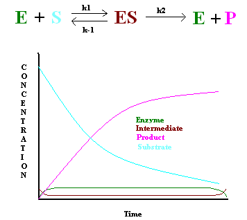
Figure 1: Steady state dynamicsin enzymes

This gives the following:

\[\dfrac{d[P]}{dt} = k_2[ES] \label{6}\]

where

\[\dfrac{d[ES]}{dt} = 0 = k_1[E][S] - k_{-1}[ES] - k_2[ES] \label{7}\]

Because

\[[S] >> [E] \label{8}\]

Using the second assumption and the fact that enzyme concentration equals the initial concentration of enzyme minus the concentration of the enzyme-substrate intermediate,

\[[E] = [E]_o - [ES] \label{9}\]

The following equation is obtained:

\[k_1[E]_o[S] = k_{-1}[ES] + k_2[ES] + k_1[ES][S] \label{10}\]

From this equation, the concentration of the ES intermediate can be found:

\[[ES] = \dfrac{k_1[E]_o[S]}{(k_{-1} + k_2) + k_1[S]} \label{11}\]

Substitute this into Equation \(\ref{3}\) gives,

\[\dfrac{d[P]}{dt} = \dfrac{k_2[E]_0[S]}{[(k_1+k_2)/k_1]+[S]} = \dfrac{k_2[E]_0[S]}{(K_M+[S]} \label{12}\]

where

\[K_M = \dfrac{k_{-1}+k_{2}}{k_1} \label{13}\]

Because in most of the cases, only the initial d[P]/dt is measured to determine the rate of product formation, (4) can be rewritten as:

\[v_0 = \dfrac{d[P]_0}{dt} = \dfrac{k_2[E]_0[S]}{K_M+[S]} \label{14}\]

Because [E]₀ = V_max/k_2. Equation \(\ref{5}\) becomes the following:

\[v_0 = \dfrac{d[P]_0}{dt} = \dfrac{k_2/k_2)v_{max}[S]}{(K_M+[S]} \label{15}\]

\[\\ = \dfrac{V_{max}[S]}{K_M+[S]} \label{16}\]

This equation is a very useful tool to in calculating v_max and K_M (the Michaelis constant), of an enzyme by using the Lineweaver-Burk plot (1/[S] vs. 1/v₀) or the Eadie-Hofstee plot (v₀/[S] vs. v₀).

Problems

Given the reaction \(A \xrightarrow[]{k_1} B \xrightarrow[]{k_2} C\)

where k₁= 0.2 M^-1s^-1 , k₂ = 2000 s^-1

1. Write the reaction rates for A, B, and C.
2. Is this a steady-state reaction?
3. Write the expression for d[C]/dt using the Steady State Approximation
4. Calculate d[C]/dt if [A] = 1M
5. Calculate [C] at t = 3 s and [A]₀ = 2M

Solutions

1) d[A]/dt = -k₁[A]; d[B]/dt = k₁[A] - k₂[B]; d[C]/dt = k₂[B]

2) Because k₁ is much larger than k₂, this is a steady state reaction.

3) d[C]/dt = k₂[B]

where d[B]/dt = k₁[A] - k₂[B] = 0

so, [B] = k₁[A]/k₂

Substitute this into d[C]/dt

d[C]/dt = k₁[A]

4) d[C]/dt = 0.2M^-1s^-1(1M) = 0.2 s^-1

5) [C] = [A]₀ (1-e^-k₁t) = 2M(1-e^-0.2(3)) = 0.9 M

References:

1. Chang, Raymond. Physical Chemistry for The Biosciences. Sausalito: University Science Books, 2005. 368-370.
2. Garrett, Reginald H, Charles M. Grisham. Biochemistry. 4^{th ed.} Boston: Brooks/Cole Cengage Learning, 2010. 389-397.
3. Segel, Irwin H. Biochemical Calculations. 2^nd ed. New Jersey: John Wiley and Sons, inc., 1976. 216-218.

Contributors

• Melanie Miner, Tu Quach, Eva Tan, Michael Cheung