Equilibrium and Le Chatelier's Principle

Objectives

• To observe the effect of an applied stress on chemical systems at equilibrium.

A reversible reaction is a reaction in which both the conversion of reactants to products (forward reaction) and the re-conversion of products to reactants (backward reaction) occur simultaneously:

Forward reaction:

\[\ce{A + B-> C + D}\]

\[\text{Reactants} \ce{->} \text{Products}\]

Backward reaction:

\[\ce{C + D -> A + B}\]

\[\text{Products} \ce{->} \text{Reactants}\]

Reversible reaction:

\[\ce{A + B <=> C + D}\]

Consider the case of a reversible reaction in which a concentrated mixture of only \(A\) and \(B\) is supplied. Initially the forward reaction rate (\(\ce{A + B -> C + D}\)) is fast since the reactant concentration is high. However as the reaction proceeds, the concentrations of \(A\) and \(B\) will decrease. Thus over time the forward reaction slows down. On the other hand, as the reaction proceeds, the concentrations of \(C\) and \(D\) are increasing. Thus although initially slow, the backward reaction rate (\(\ce{C + D -> A + B}\)) will speed up over time. Eventually a point will be reached where the rate of the forward reaction will be equal to the rate of the backward reaction. When this occurs, a state of chemical equilibrium is said to exist. Chemical equilibrium is a dynamic state. At equilibrium both the forward and backward reactions are still occurring, but the concentrations of \(A\), \(B\), \(C\), and \(D\) remain constant.

A reaction at equilibrium can be disturbed ("restarted", if you will, even tough the forward and reverse reactions never stop) if a "stress" is applied to it. Examples of stresses include increasing or decreasing concentrations or reactants or products, or temperature changes. If such a stress is applied, the reversible reaction will undergo a shift (show a net reaction) in order to re-establish equilibrium. This is known as Le Chatelier’s Principle.

Consider a hypothetical reversible reaction already at equilibrium: \(\ce{A + B <=> C + D}\). If, for example, the concentration of \(A\) is increased, the system would no longer be at equilibrium. The rate of the forward reaction (\(\ce{A + B -> C + D}\)) would briefly increase in order to reduce the amount of \(A\) present and would cause the system to undergo a net shift to the right. Eventually the forward reaction would slow down and the forward and backward reaction rates become equal again as the system returns to a state of equilibrium.

Using similar logic, the following changes in concentration are expected to cause the following shifts:

• Increasing the concentration of \(A\) or \(B\) causes a shift to the right.
• Increasing the concentration of \(C\) or \(D\) causes a shift to the left.
• Decreasing the concentration of \(A\) or \(B\) causes a shift to the left.
• Decreasing the concentration of \(C\) or \(D\) causes a shift to the right.

In other words, if a chemical is added to a reversible reaction at equilibrium, a net reaction away from the added chemical occurs. When a chemical is removed from a reversible reaction at equilibrium, a net reaction towards the removed chemical occurs.

You can also explain this using the concepts of reaction quotient Q and equilibrium constant K. At equilibrium, Q = K. In the absence of products, Q is zero, and the reaction will go forward, gradually increasing Q until it is equal to K. At this point, we are at equilibrium, all reactants and products are present, and there is no net reaction in either direction. Changing any concentration after the reaction reached equilibrium will change Q, but not K. As a consequence, we are no longer at equilibrium, and we will observe a net reaction until we reach equilibrium (and Q is equal to K again). The equilibrium concentrations at that point will be different for the initial equilibrium concentrations, but Q will have the same value again.

A change in temperature will also cause a reversible reaction at equilibrium to undergo a shift. The direction of the shift depends on whether the reaction is exothermic or endothermic. In exothermic reactions, heat energy is released and can thus be considered a product. In endothermic reactions, heat energy is absorbed and thus can be considered a reactant.

Exothermic:

\[\ce{A + B <=> C + D +} \text{ heat}\]

Endothermic:

\[\ce{A + B +} \text{ heat} \ce{<=> C + D}\]

As a general rule, if the temperature is increased, a shift away from the side of the equation with “heat” occurs. If the temperature is decreased, a shift towards the side of the equation with “heat” occurs.

If we try to explain this with Q vs K, it turns out that the equilibrium constant is not constant after all but is temperature-dependent. So K changes, and Q adjusts to match it. 

In this lab, the effect of applying stresses to a variety of chemical systems at equilibrium will be explored. The equilibrium systems to be studied are given below:

1. Saturated Sodium Chloride Solution
   \[\ce{NaCl (s) <=> Na+ (aq) + Cl^{-}  (aq)}\]
2. Aqueous Ammonia Solution (with phenolphthalein)
   \[\underbrace{\ce{NH3 (aq) }}_{\text{Clear}}\ce{+ H2O (l) <=> NH4^+ (aq) +}  \underbrace{\ce{OH^{-} (aq) }}_{\text{Pink}}\]
3. Cobalt(II) Chloride Solution
   \[\underbrace{\ce{Co(H2O)6^2+ (aq) }}_{\text{Pink}} + \ce{4 Cl^{-} (aq) <=> } \underbrace{\ce{CoCl4^2- (aq) }}_{\text{Blue}} + \ce{6 H2O (l) }\]
4. Iron(III) Thiocyanate Solution
   \[\underbrace{\ce{Fe^3+(aq) }}_{\text{Pale Yellow}} +\underbrace{\ce{SCN^{-}(aq) }}_{\text{Colorless}} \ce{<=> } \underbrace{\ce{Fe(SCN)^2+(aq) }}_{\text{Deep Red}}\]

By observing the changes that occur (color changes, precipitate formation, etc.) the direction of a particular shift may be determined. Such shifts may then be explained by carefully examining the effect of the applied stress as dictated by Le Chatelier’s Principle. If no visible changes happen, you can assume the reaction is at equilibrium. At equilibrium, you don't see the effects of forward and reverse reactions because they occur at equal rates.

Procedure

Materials and Equipment

Equipment: 10 small test tubes, test tube rack, test tube holder, hot plate, 2 medium-sized beakers (for stock solutions), 10-mL graduated cylinder, wash bottle, stirring rod, and scoopula. Sparkling water.

Chemicals: solid \(\ce{NH4Cl}\) (s), saturated \(\ce{NaCl}\) (aq), concentrated 12 M \(\ce{HCl}\) (aq), 0.1 M \(\ce{FeCl3}\) (aq), 0.1 M \(\ce{KSCN}\) (aq), 0.1 M \(\ce{AgNO3}\) (aq), 0.1 M \(\ce{CoCl2}\) (aq), concentrated 15 M \(\ce{NH3}\) (aq), phenolphthalein, 6 M \(\ce{HNO3}\) (aq), and 10% \(\ce{NaOH}\) (aq).

Safety

All of the acids and bases used in this experiment (\(\ce{NH3}\), \(\ce{HCl}\), \(\ce{HNO3}\) and \(\ce{NaOH}\)) can cause chemical burns. In particular, concentrated 12 M \(\ce{HCl}\) is extremely dangerous! If any of these chemicals spill on you, immediately rinse the affected area under running water and notify your instructor. Also note that direct contact with silver nitrate (\(\ce{AgNO3}\)) will cause dark discolorations to appear on your skin. These spots will eventually fade after repeated rinses in water. Finally, in Part 3 you will be heating a solution in a test tube directly in a Bunsen burner flame. If the solution is overheated it will splatter out of the tube, so be careful not to point the tube towards anyone while heating.

Experimental Procedure

Record all observations on your report form. These should include, but not be limited to, color changes and precipitates. Note that solution volumes are approximate for all reactions below. Dispose of all chemical waste in the containers in the hood.

Part 1: Saturated Sodium Chloride Solution

1. Place 3 mL of saturated \(\ce{NaCl}\) (aq) into a small test tube. Add one tiny crystal of NaCl to make sure it is saturated.
2. Carefully add concentrated 12 M \(\ce{HCl}\) (aq) drop-wise to the solution in the test tube until a distinct change occurs (don't add more than 3 drops). Record your observations.

Think about the following: In step 1, did the added crystal dissolve? Is this at equilibrium? In step 2, which concentrations changed, and in what direction? What was the net direction of the reaction you observed? How can you tell whether the reaction is at equilibrium again?

Part 2: Aqueous Ammonia Solution

Instructor Prep: At the beginning of lab prepare a stock solution of aqueous ammonia. Add 4 drops of concentrated 15 M \(\ce{NH3}\) (aq) and 3 drops of phenolphthalein to a 150-mL (medium) beaker, top it up with 100-mL of distilled water, and mix with a stirring rod. Label the beaker and place it on the front desk. The entire class will then use this stock solution in Part 2.

1. Place 3-mL of the prepared stock solution into a small test tube.
2. Add a medium scoop of \(\ce{NH4Cl}\) powder to the solution in this test tube. Record your observations.

Think about the following: In step 1, how do you know the reaction is at equilibrium? In step 2, which concentrations changes, and in what direction? What was the net direction of the reaction you observed? How can you tell whether the reaction is at equilibrium again? In part 1, we changed the volume of the solution a bit by adding drops of another aqueous solution. What happened to the volume of the solution in part 2? 

Part 3: Cobalt(II) Chloride Solution

1. Label three small test tubes 1-3. Place 3 mL of 0.1 M \(\ce{CoCl2}\) (aq) into tubes #1 and #3, and 1 mL into tube #2.
2. The solution in test tube #1 remains untouched. It is a control for comparison with other tubes.
3. To the solution in test tube #2, carefully add concentrated 12 M \(\ce{HCl}\) (aq) drop-wise until a drastic color change occurs. Record your observations.
4. To the solution in test tube #3, first add a medium scoop of solid \(\ce{NH4Cl}\). Then heat this solution in the provided hot water bath for about 30 seconds, or, until a distinct change occurs. Record your observations. Then cool the solution in test tube #3 back to room temperature by holding it under running tap water (or water ice slush), and again record your observations.

Think about the following: What is the evidence that tube #1 is at equilibrium? Which concentration changed in tube #2, and in which net direction did the reaction proceed? Which concentration changed in tube #3, and in which net direction did the reaction proceed before heating? Is the reaction endothermic or exothermic based on the color change upon heating and cooling?

Part 4: Iron(III) Thiocyanate Solution

Instructor Prep: At the beginning of lab prepare a stock solution of iron(III) thiocyanate. Add 2.5 mL of 0.1 M \(\ce{FeCl3}\) (aq) and 2.5 mL of 0.1 M \(\ce{KSCN}\) (aq) to a 400-mLbeaker, top it up with 250 mL of distilled water, and mix with a stirring rod. Label the beaker and place it on the front desk. The entire class (up to 18 students) will then use this stock solution in Part 4.

1. Place 3 mL each of the prepared stock solution into 4 small test tubes. Label these test tubes 1-4.
2. The solution in test tube #1 remains untouched. It is a control for comparison with other tubes.
3. To the solution in test tube #2, add 1 mL of 0.1 M \(\ce{FeCl3}\) (aq). Record your observations.
4. To the solution in test tube #3, add 1 mL of 0.1 M \(\ce{KSCN}\) (aq). Record your observations.
5. To the solution in test tube #4, add 0.1 M \(\ce{AgNO3}\) (aq) drop-wise until all the color disappears. A light precipitate may also appear. Record your observations. Here the added silver nitrate is effectively removing thiocyanate ions from the equilibrium system via a precipitation reaction:

\[\ce{Ag^{+1} (aq) + SCN^{-1} (aq) -> AgSCN (s)}\].

Think about the following: In step 3, which concentration changed, and in which net direction did the reaction proceed? What about in step 4 and step 5?

Part 5: \(\ce{CO2}\) dissolved in water

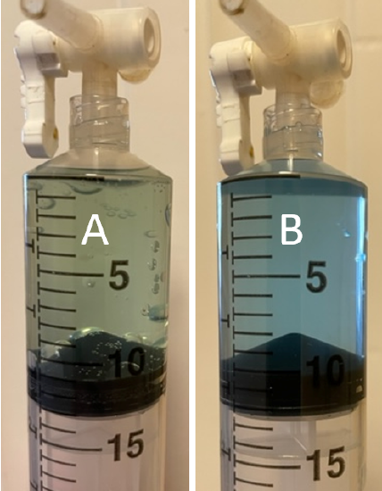
Predict the outcomes of the following experiments before approaching the "soda station" and testing your predictions. At the soda station, there are syringes with stoppers, a supply of soda with some pH indicator dissolved in it (not for human consumption!). The color of the indicator is greenish at the pH of the sparkling water, and blueish in pure water (compare panel A and panel B of the figure below).

The reaction you will study is

\[\ce{CO2(aq) <=> CO2(g)}\]

We can increase the concentration of carbon dioxide in the gas phase by pushing down the plunger, and decrease it by pulling out the plunger (or exchanging the gas in the syringe with air from the lab). We can decrease the concentration of carbon dioxide in the soda by mixing it vigorously in an open container (you know this: soda in an open container eventually "goes flat").

We can see that the reaction goes forward when we see bubbles rising out of the soda. We can estimate the concentration of carbon dioxide in solution by looking at the color of the pH indicator. The more carbon dioxide is dissolved, the more acidic the solution is. The simplified chemical equation for this is

\[\ce{CO2(aq) + H2O <=> HCO3^{-}(aq) + H+(aq)}\]

Predictions and procedures, Part 5

For the following, predict what happens (what is the direction of the net reaction, and what will happen to the color of the solution and the volume of gas in the syringe).

1. Get a 30 mL syringe. Pull up 10 mL of soda with indicator, cap the syringe, observe and record the color, and record the volume of gas, if any.
2. Pull out the plunger to the 30 mL mark, and shake the syringe. Release the plunger and, observe and record the color, and record the volume of gas.
3. Press in the plunger as far as you can with medium force, shake the syringe. Release the plunger and, observe and record the color, and record the volume of gas.
4. Repeat this a couple of times: Pull out the plunger, shake, open the valve, push the plunger in to the 10 mL mark, close the valve. Observe and record the color.

Once you have written all of your predictions on the data sheet, find a partner and do the experiment after sharing your prediction. If you have time, watch this video after you are done: https://youtu.be/QtCRxvCxa6M