1.7: Equilibria in Biochemical Systems

In this chapter we extend the concept of the Gibbs energy to mixtures. In the case of mixtures, the number of moles of the different components can change as a result of a chemical reaction or a phase transition. The partial molar Gibbs energy or chemical potential can be used to determine the spontaneity of a chemical reaction or of a phase transition. We first derive an expression for the chemical potential of gases, volatile liquids, and ideal solutions. We then introduce the concept of the activity to write a general expression for the chemical potential. For a reaction, the reaction quotient can be expressed in terms of the activities of the constituent species. Finally, we express the equilibrium constant in terms of the change in Gibbs free energy.

Learning Objectives

• Know the definition of the chemical potential as the partial molar Gibbs energy, and be able to analyze the spontaneity of a phase transition based on the change in chemical potential.
• Be able to use the chemical potential to calculate the change in Gibbs energy for a process involving changing number of moles.
• Understand the definition of the activity and how it can be used to describe both ideal and real solutions.
• Be able to write the reaction quotient in terms of the activities and modalities of the components of a reaction.
• Be able to use relation between the standard change in Gibbs energy and the equilibrium constant.

Gibbs energy and phase equilibria

For a phase transition in equilibrium at the phase transition temperature, such as the freezing of liquid water at 0 °C, the process is reversible. At equilibrium, the change in the molar Gibbs energy \(\Delta \bar{G} =0\), meaning that if two phases are at equilibrium,

\[\bar{G}_{solid} = \bar{G}_{liquid}\]

Notice here that the molar Gibbs, \(\bf{\bar{G}}\) is the same between the two phases. The molar Gibbs energy is an intensive variable (Gibbs energy per mole). We must use the molar Gibbs because the phase equilibrium is independent on the amount of substance. For example, we could have a small ice cube in equilibrium with a large volume of water at 0 °C.

If we have multiple species in our system, the intensive variable of interest is the partial molar Gibbs energy that is defined for the \(i\)th component of the system as:

\[\bar{G}_i = \left(\frac{\partial G}{\partial n_i}\right)_{T,P,n_j}\label{EQ:partialGibbs}\]

where \(n_i\) is the number of moles of the \(i\)th component, and \(n_j\) is the number of moles of all the other components in the system. The total Gibbs energy is a function of the number of moles of each species:

\[G=\sum_i \bar{G}_i n_i\label{G_sum}\]

The partial molar Gibbs, \(\bar{G}_i\) shows how infinitesimal changes in the Gibbs energy, \(\bf{dG}\), depend on infinitesimal changes in the number of moles of a component (\(n_1\), \(n_2\), …)

\[dG = \bar{G}_1 dn_1 + \bar{G}_2 dn_2 + …\label{EQ:totalGibbs}\]

The chemical potential

The partial molar Gibbs is an important property for determining phase equilibria. We give this quantity a special name called the chemical potential which gets the Greek symbol \(\mu\), and we write the chemical potential of the \(i\)th component as:

\[\mu_i = \bar{G}_i = \left(\frac{\partial G}{\partial n_i}\right)_{T,P,n_j}\label{EQ:mu}\]

Substituting Equation \ref{EQ:mu} into Equation \ref{EQ:totalGibbs} gives:

\[\begin{eqnarray}dG &=& \mu_1 dn_1 + \mu_2 dn_2 + … \nonumber \\[4pt] dG &=& \sum_i \mu_i dn_i\label{EQ:mu2}\end{eqnarray}\]

Consider the spontaneous transfer of some moles of a molecule from state A to state B as shown in Figure I.7.A.

Figure I.7.A. The conversion of a molecule from state A into state B. The number of moles converted from state A into state B is given by \(dn_B\), and is equal and opposite to \(dn_A\).

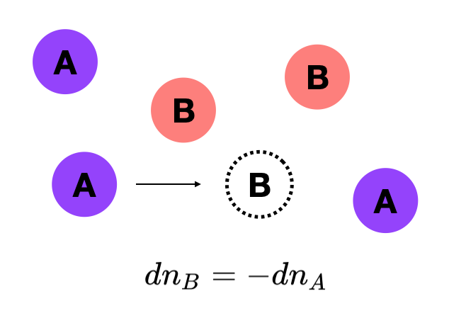
The change in the number of moles in state A, \(dn_A\) will be equal and opposite to the change in the number of moles in state B, \(dn_B\), so we can write the total change in Gibbs energy from Equation \ref{EQ:mu2} as

\[\begin{eqnarray}dG &=& \mu_A dn_A + \mu_B dn_B \nonumber \\[4pt] dG &=& (\mu_B-\mu_A) dn_B\label{EQ:mu_transfer}\end{eqnarray}\]

We now ask ourselves, when will the transition from state A into state B become spontaneous? For a spontaneous process \(dG < 0.\) Thus, the transition of \(dn_B\) moles from state A to state B, will be spontaneous if

\[\begin{eqnarray}(\mu_B-\mu_A) dn_B &<& 0 \nonumber \\[4pt] \mu_B &<& \mu_A\label{EQ:mu_matterflow}\end{eqnarray}\]

We see from Equation \ref{EQ:mu_matterflow} that matter flows in the direction of lower chemical potential.

Key Result: Matter flows spontaneously from high chemical potential to low chemical potential. The flow of matter will continue until the chemical potentials are equal, which is the equilibrium condition.

See Practice Problem 1

Recall that in Chapter I.6 we calculated the pressure dependence of the Gibbs energy for an ideal gas (See Equation I.6.33):

\[\bar{G} = \bar{G}^{\circ} + RT \ln \left(\frac{P}{P_0}\right)\label{EQ:gas}\]

where \(P_0\) is the pressure at standard conditions (1 bar). For a multi-component system of ideal gases, the partial molar Gibbs energy for each component is related to the partial pressure \(P_i\) of each species from Equation \ref{EQ:gas}:

\[\begin{eqnarray}\bar{G}_i &=& \bar{G}_i^{\circ} + RT \ln \left(\frac{P_i}{P_0}\right) \nonumber \\[4pt] \mu_i &=& \mu_i^{\circ} + RT \ln \left(\frac{P_i}{P_0}\right)\label{EQ:gas2}\end{eqnarray}\]

Notice that Equation \ref{EQ:gas2} gives an expression for the chemical potential of each species in the mixture, \(\mu_i\), given the chemical potential at the standard state \(\mu_i^{\circ}\) and the partial pressures \(P_i\).

Key Result: For a mixture of ideal gases, the chemical potential of the \(i\)th species is \(\mu_i = \mu_i^{\circ} + RT \ln \left(\frac{P_i}{P_0}\right)\) where \(P_i\) is the partial pressure of the gas and \(\mu_i^{\circ}\) is the standard chemical potential of component \(i\) when its partial pressure is 1 bar.

Thermodynamics of mixing volatile liquids

Figure I.7.B shows a pure liquid at equilibrium with its vapor in a closed container.

Figure I.7.B.

Since the system is at equilibrium the chemical potentials (partial molar Gibbs energy) are equal:

\[\mu^*_{vapor} = \mu^*_{liquid}\]

where the asterisk (*) indicates a pure substance. From Equation \ref{EQ:gas} for the gas phase we can write:

\[\mu^*_{vapor} = \mu^*_{liquid} = \mu^{\circ}_{vapor} + RT \ln \left(\frac{P^*}{\text{1 bar}}\right)\label{EQ:purliquid}\]

where \(P^*\) is the vapor pressure and \(\mu^{\circ}_{vapor}\) is the chemical potential at \(P^*\) = 1 bar.

Now consider a mixture of volatile liquids as shown in Figure I.7.C.

Figure I.7.C.

Since both components are in equilibrium with their vapors, the chemical potential for each component is still equal in the two phases. For example, for component A, we have:

\[\mu_A (l) = \mu_A (g) = \mu^{\circ}_A (g) + RT \ln \left(\frac{P_A}{\text{1 bar}}\right)\label{EQ:mixture1}\]

where \(P_A\) is the partial pressure of vapor A. Because, \(\mu^{\circ}_{vapor} = \mu^{\circ}_A (g)\), we subtract Equation \ref{EQ:purliquid} from Equation \ref{EQ:mixture1} to obtain:

\[\begin{eqnarray}\mu_A (l) – \mu^*_A (l) &=&RT \ln \left(\frac{P_A}{\text{1 bar}}\right) -RT \ln \left(\frac{P^*}{\text{1 bar}}\right) \nonumber \\[4pt] \mu_A (l) &=&\mu^*_A (l) + RT \ln \left(\frac{P_A}{P^*}\right)\label{EQ:mixture2}\end{eqnarray}\]

Thus, from Equation \ref{EQ:mixture2}, the chemical potential of a liquid in a mixture, \(\mu_A (l)\), is given in terms of the chemical potential of the pure liquid (\(\mu^*_A (l)\)) and the ratio of the vapor pressure in the pure state over the vapor pressure in the mixture.

The relationship between the two vapor pressures in Equation \ref{EQ:mixture2} is given by Raoult’s law which states that the vapor pressure of a substance in a mixture is the product of its vapor pressure as a pure liquid and its mole fraction:

\[P_A = x_A P^*\label{EQ:Raoult}\]

where \(x_A\) is the mole fraction of component A in the mixture. Inserting Equation \ref{EQ:Raoult} into Equation \ref{EQ:mixture2} gives the final expression for the chemical potential of a liquid in a mixture:

\[\mu_A (l) = \mu_A^* (l) + RT \ln x_A\label{EQ:mixture3}\]

Key Result: For a volatile liquid in a mixture, the chemical potential of component A is given by \(\mu_A (l) = \mu_A^* (l) + RT \ln x_A\) where \(\mu_A^* (l)\) is the chemical potential of the pure liquid and \(x_A\) is the mole fraction.

See Practice Problems 2 and 3

Thermodynamics of ideal solutions

For the case of a solute dissolved in a solvent (liquid), the chemical potential of the solvent is the same as for a mixture of volatile liquids:

\[\mu_{solvent} (l) = \mu_{solvent}^* (l) + RT \ln x_{solvent}\]

For the case of the solute, it is often more convenient to express the chemical potential in terms of the molality \(m\) defined as

\[\text{molality} = \frac{\text{moles of solute}}{\text{mass of solvent in kg}} \nonumber\]

For the solute, the chemical potential is:

\[\mu_{solute} (l) = \mu_{solute}^{\circ}(l) + RT \ln \left( \frac{m_{solute}}{m^{\circ}}\right)\]

Note here the careful choice of the reference state for the solute. The references state is defined as a state of unit molality where \(m^{\circ} = 1\) mol kg\(^{-1}\).

Thermodynamics of real solutions

Typically, the conditions inside the cell are far from the conditions of an ideal solution. In general, we can write an expression for the chemical potential as:

\[\mu_i = \mu^{\circ}_i + RT \ln a_i\]

where \(a_i\) is called the activity and \(\mu^{\circ}_i\) is a reference state. For real solutions, the activity is given as

\[a_i = \gamma_i (m_i/m^{\circ})\label{EQ:mu_general}\]

where \(\gamma_i\) is called the activity coefficient that is a measure of the deviation from ideality. For an ideal solution, \(\gamma = 1\) and \(a_i \rightarrow m_i/m^{\circ}\). Table I.7.i summarizes the expression of the activity and standard state for various substances. Note that for a pure sold and a pure liquid the activity is one.

Table I.7.i. Activity and standard state for various substances.

Substance	Standard State (\(\mu^{\circ}\))	activity (a)
solid	pure solid, 1 bar	1
liquid	pure liquid, 1 bar	1
gas	pure gas, 1 bar	\(P^*\)/(1 bar)
solvent	pure solvent	mole fraction \(x_i\)
ideal solute	molality of 1 mol kg\(^{-1}\)	\(m_i / m^{\circ}\)
real solution	molality of 1 mol kg\(^{-1}\)	\(\gamma_i\) \((m_i / m^{\circ})\)

The reaction quotient and chemical equilibrium

Consider a reaction in which the forward and reverse reaction can occur:

where \(a\) and \(b\) are the stoichiometric coefficients. The total change in the Gibbs energy from Equation \ref{EQ:mu2} is

\[\Delta G = b \mu_B – a \mu_A\label{EQ:Gibbs1}\]

Substituting Equation \ref{EQ:mu_general} into Equation \ref{EQ:Gibbs1} gives:

\[\begin{eqnarray}\Delta G &=& b \mu^{\circ}_B – a \mu^{\circ}_A + bRT \ln a_B – a RT \ln a_A \nonumber \\[4pt] \Delta G &=& \Delta G^{\circ} + RT \ln \left(\frac{a_B^b}{a^a_A}\right) \nonumber \\[4pt] \Delta G &=& \Delta G^{\circ} + RT \ln Q\label{EQ:Gibbs2}\end{eqnarray}\]

where

\[Q = \left(\frac{a_B^b}{a^a_A}\right)\]

is the reaction quotient and

\[\Delta G^{\circ} = b \mu^{\circ}_B – a \mu^{\circ}_A\]

is the change in Gibbs energy at standard conditions. The reaction quotient tells us which direction of the reaction will be favored. Let \(K_{eq}\) be the equilibrium constant. If \(Q < K_{eq}\), then the forward reaction will be favored. If \(Q > K_{eq}\), then the reverse reaction will be favored, and at equilibrium \(Q = K_{eq}\).

Recall that at equilibrium \(\Delta G =0\). Inserting this result into Equation \ref{EQ:Gibbs2} gives the result:

\[\Delta G^{\circ} = -RT \ln K_{eq}\label{EQ:equil}\]

where we have use the fact that at equilibrium \(Q = K_{eq}\).

See Practice Problems 4 and 5

The equilibrium constant

At equilibrium, \(K_{eq}=Q\), so the equilibrium constant can be written in terms of the activities of each species as:

\[K_{eq} = \frac{a_B^b}{a^a_A}\label{Keq1}\]

For a real solution, because \(a = \gamma (m/m^{\circ})\) we can write the equilibrium constant as:

\[\begin{eqnarray}K_{eq} &=& \frac{\gamma_B^b}{\gamma_A^a}\frac{(m_B/m^{\circ})^b}{(m_A/m^{\circ})^a} \nonumber \\[4pt] &=& K_{\gamma} K_{obs}\label{Keq2}\end{eqnarray}\]

where \(K_{obs}\) is the apparent or observed equilibrium constant given by

\[K_{obs} = \frac{(m_B/m^{\circ})^b}{(m_A/m^{\circ})^a}\label{Keq1a}\]

and \(K_{\gamma}\) is a correction for non-ideal solutions given by \((\gamma_B^b/\gamma_A^a).\) For an ideal solution \(\gamma = 1\) and the thermodynamic equilibrium constant \(K_{eq}=K_{obs}.\) Often, we express the solute concentrations in molarities (moles/L) instead of molalities. If we redefine the reference state to be 1 molar, we obtain the more familiar form of the equilibrium constant:

\[K_{eq} = \frac{[B]^b}{[A]^a}\label{Keq1b}\]

where the square bracket indicates a concentration in units of mol L\(^{-1}\).

See Practice Problem 6

Temperature dependence of \(K_{eq}\)

At standard state conditions the equilibrium constant is given by Equation \ref{EQ:equil}

\[\ln K_{eq} = -\frac{\Delta G^{\circ}}{RT}\label{EQ:T1}\]

Inserting the relation \(\Delta G^{\circ} = \Delta H^{\circ} – T \Delta S^{\circ}\) at two different temperatures \(T_1\) and \(T_2\) gives the van ‘t Hoff equation:

\[\ln \frac{K_2}{K_1} = \frac{\Delta H^{\circ} }{R} \left(\frac{1}{T_1} – \frac{1}{T_2}\right)\label{EQ:vantHoff}\]

It follows from Equation \ref{EQ:vantHoff}

\[\ln K_{eq} = -\frac{\Delta H^{\circ} }{RT} + \frac{\Delta S^{\circ}}{R}\label{EQ:vantHoff2}\]

From Equation \ref{EQ:vantHoff2} we see that a plot of \(\ln K\) vs. \(1/T\) gives a straight line with a slope of \(-\Delta H^{\circ}/R\) and an intercept of \(\Delta S^{\circ}/R\).

See Practice Problem 7

Practice Problems

Problem 1. Which of the following has a higher chemical potential? (If neither, answer “same”)

(a) H₂O (l) or H₂O (s) at water’s normal melting point (0 ºC).

(b) H₂O (l) or H₂O (s) at -5 ºC and 1 bar.

Problem 2. Which would have the higher chemical potential? Benzene at 25 ºC and 1 bar or benzene in a 0.1 M toluene solution at 25 ºC and 1 bar.

Problem 3. Calculate the chemical potential of ethanol in solution relative to that of pure ethanol when its mole fraction is 0.40 at its boiling point (78.3 ºC.)

Problem 4. The first step in the metabolic breakdown of glucose is its phosphorylation to G6P:

glucose (aq) + P_i → G6P (aq)

The standard Gibbs energy for the reaction is +14.0 kJ/mol at 37 ºC. What is the equilibrium constant? Hint: \(\Delta G^{\circ} = -RT \ln K_{eq}\).

Problem 5. Consider a motor protein (such as the F₀F₁ ATP synthase) that converts the free energy of ATP hydrolysis into mechanical work. The reaction is ATP → ADP + P_i which has a \(\Delta G^{\circ}\) = −30 kJ/mol. Under experimental conditions at T = 298 K, [ATP] = [P_i] = 10⁻³ M and [ADP] = 10⁻⁴ M. What is \(\Delta G\) of the reaction under these conditions?

Problem 6. For the following reaction, (a) write an expression for the (thermodynamic) equilibrium constant in terms of the activities of each species, (b) write an expression for the apparent (observed) equilibrium constant (\(K_{obs}\)).

CH₃COOH (aq) + H₂O (l) ↔ CH₃COO^– (aq) + H₃O⁺ (aq)

Problem 7. Consider the plot below that shows the temperature dependence of the equilibrium constant for a particular reaction. Is the reaction endothermic, exothermic, or neither?