
7.2: The Variational Method
- Page ID
- 143005
\( \newcommand{\vecs}[1]{\overset { \scriptstyle \rightharpoonup} {\mathbf{#1}} } \)
\( \newcommand{\vecd}[1]{\overset{-\!-\!\rightharpoonup}{\vphantom{a}\smash {#1}}} \)
\( \newcommand{\id}{\mathrm{id}}\) \( \newcommand{\Span}{\mathrm{span}}\)
( \newcommand{\kernel}{\mathrm{null}\,}\) \( \newcommand{\range}{\mathrm{range}\,}\)
\( \newcommand{\RealPart}{\mathrm{Re}}\) \( \newcommand{\ImaginaryPart}{\mathrm{Im}}\)
\( \newcommand{\Argument}{\mathrm{Arg}}\) \( \newcommand{\norm}[1]{\| #1 \|}\)
\( \newcommand{\inner}[2]{\langle #1, #2 \rangle}\)
\( \newcommand{\Span}{\mathrm{span}}\)
\( \newcommand{\id}{\mathrm{id}}\)
\( \newcommand{\Span}{\mathrm{span}}\)
\( \newcommand{\kernel}{\mathrm{null}\,}\)
\( \newcommand{\range}{\mathrm{range}\,}\)
\( \newcommand{\RealPart}{\mathrm{Re}}\)
\( \newcommand{\ImaginaryPart}{\mathrm{Im}}\)
\( \newcommand{\Argument}{\mathrm{Arg}}\)
\( \newcommand{\norm}[1]{\| #1 \|}\)
\( \newcommand{\inner}[2]{\langle #1, #2 \rangle}\)
\( \newcommand{\Span}{\mathrm{span}}\) \( \newcommand{\AA}{\unicode[.8,0]{x212B}}\)
\( \newcommand{\vectorA}[1]{\vec{#1}} % arrow\)
\( \newcommand{\vectorAt}[1]{\vec{\text{#1}}} % arrow\)
\( \newcommand{\vectorB}[1]{\overset { \scriptstyle \rightharpoonup} {\mathbf{#1}} } \)
\( \newcommand{\vectorC}[1]{\textbf{#1}} \)
\( \newcommand{\vectorD}[1]{\overrightarrow{#1}} \)
\( \newcommand{\vectorDt}[1]{\overrightarrow{\text{#1}}} \)
\( \newcommand{\vectE}[1]{\overset{-\!-\!\rightharpoonup}{\vphantom{a}\smash{\mathbf {#1}}}} \)
\( \newcommand{\vecs}[1]{\overset { \scriptstyle \rightharpoonup} {\mathbf{#1}} } \)
\( \newcommand{\vecd}[1]{\overset{-\!-\!\rightharpoonup}{\vphantom{a}\smash {#1}}} \)
\(\newcommand{\avec}{\mathbf a}\) \(\newcommand{\bvec}{\mathbf b}\) \(\newcommand{\cvec}{\mathbf c}\) \(\newcommand{\dvec}{\mathbf d}\) \(\newcommand{\dtil}{\widetilde{\mathbf d}}\) \(\newcommand{\evec}{\mathbf e}\) \(\newcommand{\fvec}{\mathbf f}\) \(\newcommand{\nvec}{\mathbf n}\) \(\newcommand{\pvec}{\mathbf p}\) \(\newcommand{\qvec}{\mathbf q}\) \(\newcommand{\svec}{\mathbf s}\) \(\newcommand{\tvec}{\mathbf t}\) \(\newcommand{\uvec}{\mathbf u}\) \(\newcommand{\vvec}{\mathbf v}\) \(\newcommand{\wvec}{\mathbf w}\) \(\newcommand{\xvec}{\mathbf x}\) \(\newcommand{\yvec}{\mathbf y}\) \(\newcommand{\zvec}{\mathbf z}\) \(\newcommand{\rvec}{\mathbf r}\) \(\newcommand{\mvec}{\mathbf m}\) \(\newcommand{\zerovec}{\mathbf 0}\) \(\newcommand{\onevec}{\mathbf 1}\) \(\newcommand{\real}{\mathbb R}\) \(\newcommand{\twovec}[2]{\left[\begin{array}{r}#1 \\ #2 \end{array}\right]}\) \(\newcommand{\ctwovec}[2]{\left[\begin{array}{c}#1 \\ #2 \end{array}\right]}\) \(\newcommand{\threevec}[3]{\left[\begin{array}{r}#1 \\ #2 \\ #3 \end{array}\right]}\) \(\newcommand{\cthreevec}[3]{\left[\begin{array}{c}#1 \\ #2 \\ #3 \end{array}\right]}\) \(\newcommand{\fourvec}[4]{\left[\begin{array}{r}#1 \\ #2 \\ #3 \\ #4 \end{array}\right]}\) \(\newcommand{\cfourvec}[4]{\left[\begin{array}{c}#1 \\ #2 \\ #3 \\ #4 \end{array}\right]}\) \(\newcommand{\fivevec}[5]{\left[\begin{array}{r}#1 \\ #2 \\ #3 \\ #4 \\ #5 \\ \end{array}\right]}\) \(\newcommand{\cfivevec}[5]{\left[\begin{array}{c}#1 \\ #2 \\ #3 \\ #4 \\ #5 \\ \end{array}\right]}\) \(\newcommand{\mattwo}[4]{\left[\begin{array}{rr}#1 \amp #2 \\ #3 \amp #4 \\ \end{array}\right]}\) \(\newcommand{\laspan}[1]{\text{Span}\{#1\}}\) \(\newcommand{\bcal}{\cal B}\) \(\newcommand{\ccal}{\cal C}\) \(\newcommand{\scal}{\cal S}\) \(\newcommand{\wcal}{\cal W}\) \(\newcommand{\ecal}{\cal E}\) \(\newcommand{\coords}[2]{\left\{#1\right\}_{#2}}\) \(\newcommand{\gray}[1]{\color{gray}{#1}}\) \(\newcommand{\lgray}[1]{\color{lightgray}{#1}}\) \(\newcommand{\rank}{\operatorname{rank}}\) \(\newcommand{\row}{\text{Row}}\) \(\newcommand{\col}{\text{Col}}\) \(\renewcommand{\row}{\text{Row}}\) \(\newcommand{\nul}{\text{Nul}}\) \(\newcommand{\var}{\text{Var}}\) \(\newcommand{\corr}{\text{corr}}\) \(\newcommand{\len}[1]{\left|#1\right|}\) \(\newcommand{\bbar}{\overline{\bvec}}\) \(\newcommand{\bhat}{\widehat{\bvec}}\) \(\newcommand{\bperp}{\bvec^\perp}\) \(\newcommand{\xhat}{\widehat{\xvec}}\) \(\newcommand{\vhat}{\widehat{\vvec}}\) \(\newcommand{\uhat}{\widehat{\uvec}}\) \(\newcommand{\what}{\widehat{\wvec}}\) \(\newcommand{\Sighat}{\widehat{\Sigma}}\) \(\newcommand{\lt}{<}\) \(\newcommand{\gt}{>}\) \(\newcommand{\amp}{&}\) \(\definecolor{fillinmathshade}{gray}{0.9}\)- Appreciate the complexity of solving muliti-electron atoms
- Characterize multi-electron interactions within shielding and penetration concepts
- Use the variational method as an approximation to study insolvable problems
- User variational method to evaluate the effective nuclear charge for a specific atom
In this section we introduce the powerful and versatile variational method and use it to improve the approximate solutions we found for the helium atom using the independent electron approximation.
The True (Experimentally Determined) Energy of the Helium Atom
The helium atom has two electrons bound to a nucleus with charge \(Z = 2\). The successive removal of the two electrons can be considered stepwise:
\[\ce{He} \xrightarrow {\textit{I}_1} \ce{He}^+ + e^-\xrightarrow {\textit{I}_2}\ce{He}^{++}+2e^-\label{7.1.1} \]
The first ionization energy \(I_1\) is the minimum energy required to remove the first electron from helium gas and is experimentally determined:
\[ \begin{align*} \textit{I}_1=-\textit{E}_{1\textit{s}}(\ce{He}) = 24.59\;eV \end{align*} \nonumber \]
While the second ionization energy, \(I_2\) can be experimentally determined, it can also be calculated exactly from the hydrogen atom solutions since \(\ce{He^{+}}\) is a hydrogen-like ion with \(Z=2\). Hence, we have
\[ \begin{align*} \textit{I}_2 &=-\textit{E}_{ 1\textit{s}}(\ce{He}^+) \\[4pt] &=\dfrac{Z^2}{2n^2} \\[4pt] &=54.42\mbox{ eV} \end{align*} \nonumber \]
The energy of the three separated particles on the right side of Equation \(\ref{7.1.1}\) is zero (by definition). Therefore the ground-state energy of helium atom is given by
\[ \begin{align*} E_{true}&=-(\textit{I}_1+\textit{I}_2) \\[4pt] &=-79.02\mbox{ eV}.\end{align*} \nonumber \]
which can be expressed in terms of the Rydberg constant (\(R_H=13.6 \; eV\)) that also describes the lowest energy of the hydrogen atom
\[E_{true} = -5.8066\,R_H \nonumber \]
We will attempt to reproduce this true value, as close as possible, by different theoretical approaches (all approximations).
The "Ignorance is Bliss" Approximation
The Hamiltonian for the Helium atom is:
\[\hat{H} = -\dfrac{\hbar^2}{2m_e}\nabla_{el_{1}}^2 -\dfrac{\hbar^2}{2m_e}\nabla_{el_{2}}^2 - \dfrac {Ze^2}{4\pi\epsilon_0 r_1} - \dfrac {Ze^2}{4\pi\epsilon_0 r_2} + \cancel{ \dfrac {e^2}{4\pi \epsilon_0 r_{12}} } \label{7.1.3} \]
If we simply ignore the electron-electron repulsion term, then Equation \ref{7.1.3} can be simplified to
\[ \begin{align} \hat{H} & \approx -\dfrac{\hbar^2}{2m_e}\nabla_{el_{1}}^2 - \dfrac {Ze^2}{4\pi\epsilon_0 r_1} - \dfrac{\hbar^2}{2m_e}\nabla_{el_{2}}^2 - \dfrac {Ze^2}{4\pi\epsilon_0 r_2} \label{7.1.3B} \\[4pt] &\approx h_1(r_1) + h_2(r_2) \label{7.1.3C} \end{align} \]
where \(h_1\) and \(h_2\) are one electron Hamiltonians for electron 1 and 2, respectively, and are just the hydrogen-like Hamiltonians. The approximation in Equation \ref{7.1.3C} is convenient since electron 1 is separable from electron 2, so that the two-electron wavefunction is approximated as a product to two one-electron wavefunctions:
\[\Psi_{total} = \psi_{el_{1}}\psi_{el_{2}} \label{7.1.4a} \]
or in braket notation
\[ | \Psi_{total} \rangle = \hat{H} | \psi_{el_1} \psi_{el_2} \rangle \label{7.1.4b} \]
With some operator algebra, something important arises - the one electron energies are additive:
\[ \begin{align*} \hat{H} \Psi_{total} &= (\hat{H}_{el_1} + \hat{H}_{el_2}) \psi_{n\ {el_1}} \psi_{n\ {el_2}} = (E_{n_1} + E_{n_2}) \psi_{n\ {el_1}} \psi_{n\ {el_2}} \end{align*} \nonumber \]
or in bra-ket notation
\[ \begin{align*} \hat{H} | \Psi_{total} \rangle &= \hat{H} | \psi_{el_1} \psi_{el_2} \rangle \\[4pt] &= (E_{n_1} + E_{n_2}) | \psi_{1} \psi_{2} \rangle \end{align*} \nonumber \]
The energy for a ground state Helium atom (both electrons in lowest state) is then
\[ \begin{align*} E_{He_{1s}} &= \underset{\text{energy of single electron in helium}}{E_{n_1}} + \underset{\text{energy of single electron in helium}}{E_{n_2}} \\[4pt] &= -R_H\left(\dfrac{Z^2}{1}\right) -R_H \left(\dfrac{Z^2}{1}\right) \\[4pt] &= -8R_H \end{align*} \nonumber \]
This approximation significantly overestimates the true energy of the helium atom \(E_{He_{1s}} = -5.8066\,R\). This is a poor approximation and we need to address electron-electron repulsion properly (or better at least).
Shielding and Penetration
One way to take electron-electron repulsion into account is to modify the form of the wavefunction. A logical modification is to change the nuclear charge, \(Z\), in the wavefunctions to an effective nuclear charge (\(Z_{eff}\)), from +2 to a smaller value. The rationale for making this modification is that one electron partially shields the nuclear charge from the other electron, as shown in Figure 7.1.1 .

A region of negative charge density between one of the electrons and the +2 nucleus makes the potential energy between them more positive (decreases the attraction between them). We can effect this change mathematically by using \(\zeta < 2\) in the wavefunction expression. If the shielding were complete, then \(Z_{eff}\) would equal 1. If there is no shielding, then \(Z_{eff}= 2\). So a way to take into account the electron-electron interaction is by saying it produces a shielding effect. The shielding is not zero, and it is not complete, so the effective nuclear charge varies between one and two.
In general, a theory should be able to make predictions in advance of knowledge of the experimental result. Consequently, a principle and method for choosing the best value for \(Z_{eff}\) or any other adjustable parameter that is to be optimized in a calculation is needed. The Variational Principle provides the required criterion and method and says that the best value for any variable parameter in an approximate wavefunction is the value that gives the lowest energy for the ground state; i.e., the value that minimizes the energy. The variational method is the procedure that is used to find the lowest energy and the best values for the variable parameters.
A Better Approximation: The Variational Method
The variational method is one way of finding approximations to the lowest energy eigenstate or ground state, and some excited states. This allows calculating approximate wavefunctions and is the variational principle. The method consists in choosing a "trial wavefunction" depending on one or more parameters, and finding the values of these parameters for which the expectation value of the energy is the lowest possible. The wavefunction obtained by fixing the parameters to such values is then an approximation to the ground state wavefunction, and the expectation value of the energy in that state is an upper bound to the ground state energy.
The variational principle means that the expectation value for the binding energy obtained using an approximate wavefunction and the exact Hamiltonian operator will be higher than or equal to the true energy for the system. This idea is really powerful. When implemented, it permits us to find the best approximate wavefunction from a given wavefunction that contains one or more adjustable parameters, called a trial wavefunction. A mathematical statement of the variational principle is
\[ E_{trial} \ge E_{true} \label {7.1.7} \]
where
\[ \begin{align} E_{trial} &= \dfrac{ \langle \psi _{trial}| \hat {H} | \psi _{trial} \rangle}{\langle \psi _{trial} | \psi _{trial} \rangle} \\[4pt] &= \dfrac {\displaystyle \int \psi _{trial} ^* \hat {H} \psi _{trial} d \tau}{\displaystyle \int \psi _{trial} ^* \psi _{trial} d\tau } \label {7.1.8} \end{align} \]
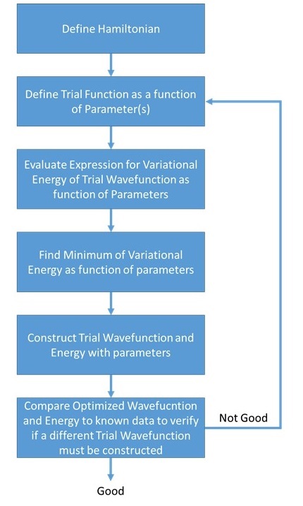
Equation \(\ref{7.1.7}\) is called the variational theorem and states that for a time-independent Hamiltonian operator, any trial wavefunction will have an variational energy (i.e., expectation value) that is greater than or equal to the true ground state wavefunction corresponding to the given Hamiltonian (Equation \ref{7.1.7}). Because of this, the variational energy is an upper bound to the true ground state energy of a given molecule. The general approach of this method consists in choosing a "trial wavefunction" depending on one or more parameters, and finding the values of these parameters for which the expectation value of the energy is the lowest possible (Figure 7.1.2 ).
The variational energy \(E_{trial}\) is only equal to the true energy \(E_{true}\) when the the corresponding trial wavefunction \(\psi_{trial}\) is equal to the true wavefunction \(\psi_{true}\).
Application to the Helium atom Ground State
Often the expectation values (numerator) and normalization integrals (denominator) in Equation \(\ref{7.1.8}\) can be evaluated analytically. For the case of the He atom, let's consider the trial wavefunction as the product wavefunction given by Equation \(\ref{7-13}\) (this is called the orbital approximation),
\[\psi (r_1 , r_2) \approx \varphi (r_1) \varphi (r_2) \label {7-13} \]
The adjustable or variable parameter in the trial wavefunction is the effective nuclear charge \(\zeta\), and the Hamiltonian is the complete form given below (Note: quantum calculations typically refer to effective nuclear charge as \(\zeta\) rather than \(Z_{eff}\) as we used previously).
\[\hat {H} = -\dfrac {\hbar ^2}{2m} \nabla^2_1 - \dfrac {\zeta e^2}{4 \pi \epsilon _0 r_1} - \dfrac {\hbar ^2}{2m} \nabla ^2_2 - \dfrac {\zeta e^2}{4 \pi \epsilon _0 r_2} + \dfrac {e^2}{4 \pi \epsilon _0 r_{12}} \label {9-9} \]
the adjustable or variable parameter in the trial wavefunction is the effective nuclear charge \(\zeta\) (would be equal to \(\zeta=2\) if fully unshielded), and the Hamiltonian is the complete form. When the expectation value for the trial energy (Equation \ref{7.1.8}) is evaluated for helium, the result is a variational energy that depends on the adjustable parameter, \(\zeta\).
\[ E_{trial} (\zeta) = \dfrac {\mu e^4}{4 \epsilon ^2_0 h} \left ( \zeta ^2 - \dfrac {27}{8} \zeta \right ) \label {7.1.9} \]
This function is plotted in Figure 7.1.3 as a function of \(\zeta\). According to the variational principle (Equation \ref{7.1.7}), the minimum value of the energy on this graph is the best approximation of the true energy of the system, and the associated value of \(\zeta\) is the best value for the adjustable parameter.

Using the mathematical function for the energy of a system, the minimum energy with respect to the adjustable parameter can be found by taking the derivative of the energy with respect to that parameter, setting the resulting expression equal to zero, and solving for the parameter, in this case \(\zeta\). This is a standard method in calculus for finding maxima and minima.
Find the value for \(\zeta\) that minimizes the helium binding energy for the product trial wavefunction in Equation \ref{7-13} with the Hamiltonian in Equation \ref{9-9}. and compare the binding energy to the experimental value. What is the percent error in the calculated value?
Solution
The variational method requires following the workflow in Figure 7.1.2 .
- Step 1: Define the Hamiltonian - This is given by Equation \ref{9-9}.
- Step 2: Define the trial wavefunction as a function of at least one parameter - This is given by Equation \ref{7-13}.
- Step 3: Evaluate variational energy (\(E_{trial}\) integral (Equation \ref{7.1.8}) - This procedure was already above in Equation \ref{7.1.9}.
- Step 4: Minimize the variational energy as a function of the parameter(s) - Following the standard approach to find extrema in calculus, evaluate the derivative of \(E_{trial}\) with respect to \(\zeta\) and set to zero: \[\dfrac{dE_{trial}}{d\zeta} = \dfrac {\mu e^4}{4 \epsilon ^2_0 h} \left ( 2 \zeta - \dfrac {27}{8} \right ) =0 \nonumber \] then find solve for the roots of this polynomial \[2 \zeta - \dfrac {27}{8}=0 \nonumber \] or \[\zeta = \dfrac {27}{16} \approx 1.6875 \nonumber \]
- Step 5-6: The question does not ask for the optimized wavefunction (Step 5) or to compare the result with the true value to evaluate the quality of the approximation (Step 6). We can skip these steps.
From Exercise 7.1.1 , the \(\zeta = 1.6875\) and the approximate energy we calculate using this approximation method, Eapprox = -77.483 eV. Table 7.1.1 show that a substantial improvement in the accuracy of the computed binding energy is obtained by using shielding to account for the electron-electron interaction. Including the effect of electron shielding in the wavefunction reduces the error in the binding energy to about 2%. This idea is very simple, elegant, and significant.
|
|
|
|---|---|
| "Ignorance is Bliss" Approximation (neglect repulsion between electrons) | -108.8 |
| Variational method with variable effective charge | -77.483 |
| Experimental | -79.0 |
The improvement we have seen in the total energy calculations using a variable parameter \(\zeta\) indicates that an important contribution of electron-electron interaction or repulsion to the total binding energy arises from the fact that each electron shields the nuclear charge from the other electron. It is reasonable to assume the electrons are independent; i.e., that they move independently, but the shielding must be taken into account in order to fine-tune the wavefunctions. The inclusion of optimizable parameters in the wavefunction allows us to develop a clear physical image of the consequences of our variation calculation. Calculating energies correctly is important, and it is also important to be able to visualize electron densities for multi-electron systems. In the next two sections, we take a temporary break from our consideration of approximation methods in order to examine multi-electron wavefunctions more closely.