Appendix A: Treatment of Experimental Errors
- Page ID
- 435125
\( \newcommand{\vecs}[1]{\overset { \scriptstyle \rightharpoonup} {\mathbf{#1}} } \)
\( \newcommand{\vecd}[1]{\overset{-\!-\!\rightharpoonup}{\vphantom{a}\smash {#1}}} \)
\( \newcommand{\dsum}{\displaystyle\sum\limits} \)
\( \newcommand{\dint}{\displaystyle\int\limits} \)
\( \newcommand{\dlim}{\displaystyle\lim\limits} \)
\( \newcommand{\id}{\mathrm{id}}\) \( \newcommand{\Span}{\mathrm{span}}\)
( \newcommand{\kernel}{\mathrm{null}\,}\) \( \newcommand{\range}{\mathrm{range}\,}\)
\( \newcommand{\RealPart}{\mathrm{Re}}\) \( \newcommand{\ImaginaryPart}{\mathrm{Im}}\)
\( \newcommand{\Argument}{\mathrm{Arg}}\) \( \newcommand{\norm}[1]{\| #1 \|}\)
\( \newcommand{\inner}[2]{\langle #1, #2 \rangle}\)
\( \newcommand{\Span}{\mathrm{span}}\)
\( \newcommand{\id}{\mathrm{id}}\)
\( \newcommand{\Span}{\mathrm{span}}\)
\( \newcommand{\kernel}{\mathrm{null}\,}\)
\( \newcommand{\range}{\mathrm{range}\,}\)
\( \newcommand{\RealPart}{\mathrm{Re}}\)
\( \newcommand{\ImaginaryPart}{\mathrm{Im}}\)
\( \newcommand{\Argument}{\mathrm{Arg}}\)
\( \newcommand{\norm}[1]{\| #1 \|}\)
\( \newcommand{\inner}[2]{\langle #1, #2 \rangle}\)
\( \newcommand{\Span}{\mathrm{span}}\) \( \newcommand{\AA}{\unicode[.8,0]{x212B}}\)
\( \newcommand{\vectorA}[1]{\vec{#1}} % arrow\)
\( \newcommand{\vectorAt}[1]{\vec{\text{#1}}} % arrow\)
\( \newcommand{\vectorB}[1]{\overset { \scriptstyle \rightharpoonup} {\mathbf{#1}} } \)
\( \newcommand{\vectorC}[1]{\textbf{#1}} \)
\( \newcommand{\vectorD}[1]{\overrightarrow{#1}} \)
\( \newcommand{\vectorDt}[1]{\overrightarrow{\text{#1}}} \)
\( \newcommand{\vectE}[1]{\overset{-\!-\!\rightharpoonup}{\vphantom{a}\smash{\mathbf {#1}}}} \)
\( \newcommand{\vecs}[1]{\overset { \scriptstyle \rightharpoonup} {\mathbf{#1}} } \)
\(\newcommand{\longvect}{\overrightarrow}\)
\( \newcommand{\vecd}[1]{\overset{-\!-\!\rightharpoonup}{\vphantom{a}\smash {#1}}} \)
\(\newcommand{\avec}{\mathbf a}\) \(\newcommand{\bvec}{\mathbf b}\) \(\newcommand{\cvec}{\mathbf c}\) \(\newcommand{\dvec}{\mathbf d}\) \(\newcommand{\dtil}{\widetilde{\mathbf d}}\) \(\newcommand{\evec}{\mathbf e}\) \(\newcommand{\fvec}{\mathbf f}\) \(\newcommand{\nvec}{\mathbf n}\) \(\newcommand{\pvec}{\mathbf p}\) \(\newcommand{\qvec}{\mathbf q}\) \(\newcommand{\svec}{\mathbf s}\) \(\newcommand{\tvec}{\mathbf t}\) \(\newcommand{\uvec}{\mathbf u}\) \(\newcommand{\vvec}{\mathbf v}\) \(\newcommand{\wvec}{\mathbf w}\) \(\newcommand{\xvec}{\mathbf x}\) \(\newcommand{\yvec}{\mathbf y}\) \(\newcommand{\zvec}{\mathbf z}\) \(\newcommand{\rvec}{\mathbf r}\) \(\newcommand{\mvec}{\mathbf m}\) \(\newcommand{\zerovec}{\mathbf 0}\) \(\newcommand{\onevec}{\mathbf 1}\) \(\newcommand{\real}{\mathbb R}\) \(\newcommand{\twovec}[2]{\left[\begin{array}{r}#1 \\ #2 \end{array}\right]}\) \(\newcommand{\ctwovec}[2]{\left[\begin{array}{c}#1 \\ #2 \end{array}\right]}\) \(\newcommand{\threevec}[3]{\left[\begin{array}{r}#1 \\ #2 \\ #3 \end{array}\right]}\) \(\newcommand{\cthreevec}[3]{\left[\begin{array}{c}#1 \\ #2 \\ #3 \end{array}\right]}\) \(\newcommand{\fourvec}[4]{\left[\begin{array}{r}#1 \\ #2 \\ #3 \\ #4 \end{array}\right]}\) \(\newcommand{\cfourvec}[4]{\left[\begin{array}{c}#1 \\ #2 \\ #3 \\ #4 \end{array}\right]}\) \(\newcommand{\fivevec}[5]{\left[\begin{array}{r}#1 \\ #2 \\ #3 \\ #4 \\ #5 \\ \end{array}\right]}\) \(\newcommand{\cfivevec}[5]{\left[\begin{array}{c}#1 \\ #2 \\ #3 \\ #4 \\ #5 \\ \end{array}\right]}\) \(\newcommand{\mattwo}[4]{\left[\begin{array}{rr}#1 \amp #2 \\ #3 \amp #4 \\ \end{array}\right]}\) \(\newcommand{\laspan}[1]{\text{Span}\{#1\}}\) \(\newcommand{\bcal}{\cal B}\) \(\newcommand{\ccal}{\cal C}\) \(\newcommand{\scal}{\cal S}\) \(\newcommand{\wcal}{\cal W}\) \(\newcommand{\ecal}{\cal E}\) \(\newcommand{\coords}[2]{\left\{#1\right\}_{#2}}\) \(\newcommand{\gray}[1]{\color{gray}{#1}}\) \(\newcommand{\lgray}[1]{\color{lightgray}{#1}}\) \(\newcommand{\rank}{\operatorname{rank}}\) \(\newcommand{\row}{\text{Row}}\) \(\newcommand{\col}{\text{Col}}\) \(\renewcommand{\row}{\text{Row}}\) \(\newcommand{\nul}{\text{Nul}}\) \(\newcommand{\var}{\text{Var}}\) \(\newcommand{\corr}{\text{corr}}\) \(\newcommand{\len}[1]{\left|#1\right|}\) \(\newcommand{\bbar}{\overline{\bvec}}\) \(\newcommand{\bhat}{\widehat{\bvec}}\) \(\newcommand{\bperp}{\bvec^\perp}\) \(\newcommand{\xhat}{\widehat{\xvec}}\) \(\newcommand{\vhat}{\widehat{\vvec}}\) \(\newcommand{\uhat}{\widehat{\uvec}}\) \(\newcommand{\what}{\widehat{\wvec}}\) \(\newcommand{\Sighat}{\widehat{\Sigma}}\) \(\newcommand{\lt}{<}\) \(\newcommand{\gt}{>}\) \(\newcommand{\amp}{&}\) \(\definecolor{fillinmathshade}{gray}{0.9}\)Every measurement that is made in the laboratory is subject to error. An experimenter should try to minimize these errors. However, since they cannot be entirely eliminated, a means to describe and quantify the errors is needed, so that another experimenter can judge and interpret the uncertainties reported with any result. This outline defines certain terms that are important in the treatment of errors. Certain conclusions that are derived from a statistical analysis of random errors are also presented. Finally, some rules are given for discarding questionable data, for propagating errors in calculations, and for finding the best straight line through a set of graphed data.
Types of Error
There are two general classes of errors. Systematic or determinate errors are reproducible in successive measurements and may be detected and corrected. Often systematic error is due to an incorrect calibration, for example of volumetric glassware, an electronic balance or a pH meter, and causes all readings to have the same recurring error. Random or indeterminate errors are due to limitations of the measurement that are beyond the experimenter's control. They cannot be eliminated, and lead to positive and negative fluctuations in successive measurements. Examples of random errors are the fluctuations in the interpolation of the reading of a thermometer scale by different observers and the oscillations in the output of a pH meter due to electrical noise.
Accuracy and Precision
The accuracy of a result refers to how close the result is to its true value, while the precision of a result indicates its reproducibility in successive measurements. If successive measurements are in close agreement, the result has a high precision, which usually implies small random errors. If the result is in good agreement with the true value, it has high accuracy, which suggests small systematic errors.
A well-designed experiment attempts to minimize both systematic and random errors, thereby
allowing both high accuracy and high precision from careful measurements. Since systematic errors are not generally manifest in successive measurements, they can be avoided only by careful calibration and consideration of all possible corrections. Random errors are indicated by the fluctuations in successive measurements. They can be quantified and treated by the methods of statistics. In the following we restrict the discussion to random errors, assuming that all systematic errors have been eliminated.
Statistical Treatment of Random Errors
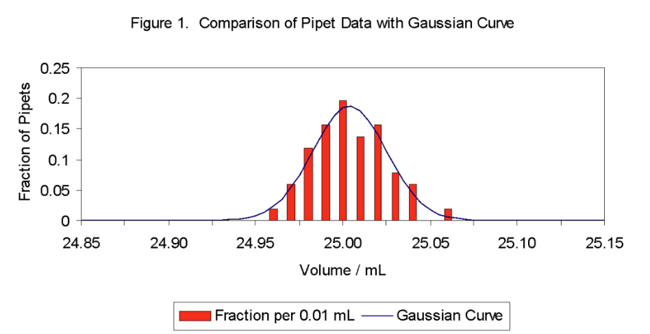
Let's consider as an example the volume of water delivered by a set of 25 mL pipets. A manufacturer produces these to deliver 25.00 mL at 20°C with a stated tolerance of ±0.03 mL. A sample of 100 pipets is tested for accuracy by measuring the delivered volumes. The column graph in Figure 1 shows the fractional number of the sampled pipets that deliver a particular volume in each 0.01 mL interval. The maximum of the column graph indicates that most of the pipets deliver between 24.995 and 25.005 mL. However, other pipets deliver lesser or greater volumes due to random variations in the manufacturing process.
The mean or average, \( \ce{x_{avg}}\), of a set of results is defined by
\( \ce{x_{avg} = \frac{\sum_{i}x_{i}}{N} } \)
where \( \ce{x_{i}}\) is an individual result and N is the total number of results. For the data in Figure 1, the mean volume is 25.0039 mL. The mean alone, however, provides no indication of the uncertainty. The same mean could have resulted from data with either more or less spread. The spread of the individual results about the mean is characterized by the sample standard deviation, s, which is given by
\( \ce{ s = ( \frac{\sum_{i} (x_{i}-x_{avg})^{2}}{N-1} )^{1/2} } \)
The pipet data has a sample standard deviation of 0.0213 mL.
The sample standard deviation gives us a quantitative measurement of the precision. To see how this works, let's imagine that we increase the number of sampled pipets. The bar graph will show less irregularities. A line connecting the tops of the bars will approach a smooth bell-shaped curve as the number of samples approaches infinity and the volume interval approaches zero. This smooth curve is called a Gaussian or normal error curve. Its formula is
\( \ce{ y(x) = \frac {1}{\sigma(2\pi)^{1/2}} exp [-\frac{(x-\mu)^{2}}{2\sigma^{2}} ] } \)
where exp[···] = e [···] with e = 2.178..., the base of natural logarithms. For an infinite or complete data set, the mean is called \( \ce{\mu}\) (the population mean) and the standard deviation \( \ce{\sigma}\) (the population standard deviation). We can never measure \( \ce{\mu}\) and \( \ce{\sigma}\), but \( \ce{x_{avg}}\) and \( \ce{s}\) approach \( \ce{\mu}\) and \( \ce{\sigma}\), respectively, as the number of samples or measurements increases. The smooth curve in Figure 1 shows a graph of equation (3) for \( \ce{\mu}\) = 25.0039 mL and \( \ce{\sigma}\) = 0.0213 mL, as approximated by \( \ce{x_{avg}}\) and \( \ce{s}\).
The Gaussian curve gives the probability of obtaining a particular result \( \ce{x}\) for a given \( \ce{\mu}\) and \( \ce{\sigma}\). This probability is proportional to the \( \ce{y}\) value of the Gaussian curve for the particular \( \ce{x}\) value. The maximum probability occurs at the maximum of the function, which corresponds to \( \ce{x=\mu}\). Other values of \( \ce{x}\) have lower probabilities. Because of the symmetry of the curve, values of \( \ce{x}\) that deviate from \( \ce{\mu}\) by the same magnitude, i.e., have the same \( \ce{|(x-\mu)|}\), have the same probabilities.
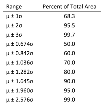
The significance of the standard deviation is that it measures the width of the Gaussian curve. The larger the value of \( \ce{\sigma}\), the broader the curve and the greater the probability of obtaining an \( \ce{x}\) value that deviates from \( \ce{\mu}\). One can calculate the percent of the samples or measurements that occurs in a given range from the corresponding fraction of the area under the Gaussian curve by integral calculus. Representative results are summarized in Table 1. For example, 68.3% of the samples or measurements are expected to lie between \( \ce{\mu-\sigma}\) and \( \ce{\mu+\sigma}\), and 90.0% between \( \ce{\mu-1.645\sigma}\) and \( \ce{\mu+1.645\sigma}\). Table 1. Area under Gaussian Curve
The manufacturer can thus have 90.0% confidence that some other pipet (from the identical manufacturing process) will deliver a volume in the range \( \ce{\mu \pm 1.645 \sigma} \). Estimating \( \ce {\mu = x_{avg} =} \)25.004 mL and \( \ce{\sigma = s =}\) 0.0213 mL, the manufacturer can claim that the pipets deliver 25.00 mL with a tolerance of (1.64)(0.021) = 0.03 mL. The 90% degree of confidence is hidden in this claim, and a higher degree of confidence would have correspondingly poorer (greater) tolerances. The purchaser, however, may not be told these details!
Confidence Limits
Although we cannot determine \(\ce{\mu}\) and \(\ce{\sigma}\) from a limited number of measurements, statistical analysis does allow us to obtain the confidence limits for \(\ce{\mu}\) from a limited data set. Namely, we can state to a certain probability (confidence) that \(\ce{\mu}\) will lie within certain limits of \(\ce{x_{avg}}\). These confidence limits (CL) are given by
\( \ce{CL = \pm \frac{ts}{\sqrt{N}}} \)
where \(\ce{s}\) is the sample standard deviation and N is the number of measurements. The \( \ce{\sqrt{N}} \) term in the denominator accounts for the fact that the sample mean has a greater precision than any individual measurement. 1*The factor t (called Student's t value) is given in Table 2 for several levels of confidence. The t-value for other levels of confidence can be calculated with a microcomputer spreadsheet using the built-in functions. In MS Excel, the function that returns t is TINV(\(\ce{\alpha}\), DF) where 1-\(\ce{\alpha}\) is the confidence level (for 95% confidence, \(\ce{\alpha}\) = 0.05) and DF is the degrees of freedom. The t-value can be viewed as a correction for the limited number of measurements in a data set and the associated errors in approximating \(\ce{\mu}\) and \(\ce{\sigma}\) by \(\ce{x_{avg}}\) and \(\ce{s}\), respectively. If N is infinite, the value of t for the various confidence limits in Table 2 equals the number multiplying \(\ce{\sigma}\) in the range column of Table 1 for the corresponding confidence. For example, for N infinite and 90.0% confidence, Table 2 gives t = 1.645. This agrees with the factor multiplying \(\ce{\sigma}\) for 90.0% confidence in Table 1. However, if N is finite, the value of t for a given confidence must increase as N decreases, since \(\ce{x_{avg}}\) and \(\ce{s}\) become poorer estimates of \(\ce{\mu}\) and \(\ce{\sigma}\).
*Imagine a group of data sets. For each set the sample mean is calculated. The group of means will show a scatter that is also described by a Gaussian curve. However, the width of this curve will be less than the width of the curve associated with a single data set; the standard deviation of the mean is less than the standard deviation of the data. The standard deviation in the mean, \(\ce{s_{x}}\), can be estimated from just one data set and its sample standard deviation, \(\ce{s}\), by \(\ce{s_{x}=\frac{s}{\sqrt{N}}}\). This means that the uncertainty in the mean decreases as the square-root of the number of measurements increases. Hence, to reduce the uncertainty in the mean by a factor of two, the number of measurements must be increased by a factor of four.
Estimates of \(\ce{\mu}\) and its confidence limits become important, say, in the calibration of an individual pipet. Let's assume that 10 determinations of the delivered volume for a particular pipet also yield \(\ce{x_{avg}=}\) 25.004 mL with \(\ce{s}\) = 0.0213 mL. The best estimate of the population mean (the mean from an infinite number of measurements of the delivered volume) is \(\ce{\mu = x_{avg} =}\)25.004 mL. Its 95.0% confidence limits for 10 measurements is then \(\ce{\pm \frac{ts}{\sqrt{N}} = \pm \frac{(2.262)(0.0213)}{\sqrt{10}}= \pm0.0152 } \) mL where the t value was obtained from Table 2. Accordingly, to 95.0% confidence the average volume of the particular pipet is 25.004 ± 0.015 mL. This means that there is a 95% probability that the true or population mean will lie within ±0.015 mL of 25.004 mL.
You will use the foregoing method of estimating the population or true mean and its confidence limits in many of your laboratory experiments. Typically you will make at least three measurements or determinations of a quantity. You will report the sample mean, \( \ce{x_{avg}} \), as an approximation of the true mean; the sample standard deviation, \( \ce{s}\) as an approximation of the population standard deviation; and the 95% confidence limits of the mean. The chosen confidence is that typically used when reporting scientific results. The mean is calculated from equation (1), the standard deviation from equation (2) and the confidence limits of the mean from equation (4) using the t values for 95% confidence in Table 2. Scientific calculators and microcomputer spreadsheets typically have built-in functions to calculate the sample mean and the sample standard deviation, but not confidence limits.
Q Test
Sometimes a single piece of data appears inconsistent with the remaining data. For example, the questionable point may be much larger or much smaller than the remaining points. In such cases, one requires a valid method to test if the questionable point can be discarded in calculating the sample mean and standard deviation. The Q test is used to help make this decision.
Assume that the outlier (the data point in question) has a value \( \ce{x_{0}} \). Calculate the magnitude of the difference between \( \ce{x_{0}} \) and its nearest value from the remaining data (called the gap), and the magnitude of the spread of the total data including the value \( \ce{x_{0}} \) (called the range). The quantity \( \ce{Q_{Data}} \), given by
\( \ce{Q_{Data} = \frac{gap}{range}} \)
is compared with tabulated critical values of Q for a chosen confidence level. If \( \ce{Q_{Data}>Q_{Critical}} \), the outlier can be discarded to the chosen degree of confidence. The Q test is fairly stringent and not particularly helpful for small data sets if high confidence is required. It is common to use a 90% confidence for the Q test, so that any data point that has less than a 10% chance of being valid can be discarded. Values of \( \ce{Q_{Critical}} \) for 90% confidence are given in Table 3.
Let's consider an example to clarify the use of the Q test. Suppose that you make four determinations of the concentration of a solution, and that these yield 0.1155, 0.1150, 0.1148 and 0.1172 M. The mean concentration is 0.1156 M with a standard deviation of 0.0011 M. The 0.1172 M data point appears questionable since it is nearly two standard deviations away from the mean. The gap is (0.1172 - 0.1155) = 0.0017, and the range is (0.1172 - 0.1148) = 0.0024, so that \( \ce{Q_{Data}} \) = 0.0017/0.0024 = 0.71. Table 3 gives \( \ce{Q_{Critical}} \) = 0.76 for 90% confidence and four determinations. Since \( \ce{Q_{Data}<Q_{Critical}} \), the questionable point cannot be discarded. There is more than a 10% chance that the questionable point is valid.
Several caveats should be noted about the Q test. Firstly, it may be applied to only one outlier of a small data set. Secondly, even at 90% confidence some "bad" data point may be retained. If you are sure that the point is bad because of some action noted during the measurement (for example, you know that you overshot the endpoint of a titration for the particular sample during its analysis), then the point can and should be discarded. Thirdly, an apparent outlier can result in a limited data set simply from the statistical distribution of random errors, as occurred in the above example. Repeating the measurement so as to increase the data set, and thereby decrease the importance of the apparent outlier, is generally much more valuable than any statistical test.
Propagation of Errors
A quantity of interest may be a function of several independent variables, say f(x,y). It would be evaluated by performing arithmetic operations with several numbers (x and y), each of which has an associated random error. These random errors, which we denote as \(\ce{e_{x}}\) and \(\ce{e_{y}}\), may be simply estimates, standard deviations or confidence limits, so long as the same measure is used for both. How do these errors propagate in determining the corresponding error, \(\ce{e_{f}}\), in the final quantity of interest? This error is not simply the sum of the individual errors since some of these are likely to be positive and others negative, so that a certain cancellation will occur. We give below the equations determining \(\ce{e_{f}}\) for simple operations. These equations are obtained using differential calculus.
\( \ce{ f = \alpha x + \beta y } \) with \(\ce{\alpha} \) and \( \ce{\beta} \) constants.
\( \ce {e_{f}^{2} = \alpha^{2}e_{x}^{2} + \beta^{2}e_{y}^{2} } \)
\( \ce{ f = \alpha x^{n}\beta y^{m} } \) with \(\ce{\alpha} \), \(\ce{n} \) and \( \ce{m} \) constants.
\( \ce { \frac{e_{f}^{2}}{f^{2}} = n^{2} (\frac{e_{x}}{x})^{2} + m^{2}(\frac{e_{y}}{y})^{2} } \)
The case \( \ce{ f = \alpha x + \beta y } \) includes addition and subtraction by choosing the signs of \(\ce{\alpha} \) and \( \ce{\beta} \), while the case \( \ce{ f = \alpha x^{n}\beta y^{m} } \) includes multiplication and division by appropriate choice of the exponents. Any of the constants \(\ce{\alpha} \), \(\ce{\beta}\), \(\ce{n} \), or \( \ce{m} \) can be positive, negative or zero. The cases where \(\ce{\beta = 0}\) or \(\ce{m = 0}\), for example, correspond to the function depending on the single variable \(\ce{(x)}\). More complicated cases, involving, for example, both addition and division, can be deduced by treating the various parts or factors separately using the given equations. Two simple examples of error propagation are considered below.
Example 1. You determine the mass (let's call this f) of a substance by first weighing a container \(\ce{(x)}\) and then the container with the substance \(\ce{(y)}\), using a balance accurate to 0.1 mg. The mass of the substance is then \(\ce{f = y ? x}\), and its error from equation (6) is
\(\ce { e_{f} = (e^{2}_{x})^{1/2} = (0.1^{2} + 0.1^{2})^{1/2} = 0.14} \) mg
since \( \ce{\alpha = \beta = 1} \) and \( \ce{ e_{x} = e_{y} = 0.1} \) mg
Example 2. You determine the density, \(\ce{d}\), of a block of metal by separate measurements of its mass, \(\ce{m}\), and volume, \(\ce{V}\). The mass and volume are each measured four times. Their mean values with standard deviations in parentheses are \(\ce{m_{avg}}\) = 54.32 (0.05) g and \(\ce{V_{avg}}\) = 6.78 (0.02) mL. The density is 54.32/6.78 = 8.012 g/mL. The standard deviation in \(\ce{d}\), \(\ce{e_{d}}\), would be calculated from equation (7), which gives
\( \ce{ e_{d} = d[(\frac{e_{m}}{m})^{2} + (\frac{e_{V}}{V})^{2}]^{1/2} } \)
\( \ce { = 8.012 [(\frac{0.05}{54.32})^{2} + (\frac{0.02}{6.78})^{2}]^{1/2} }\)
\( \ce{ 8.012(0.00309) = 0.025 } \) g/mL
We can also obtain the 95% confidence limits for the true density by using the 95% confidence limits for the mass and volume. For four measurements or three degrees of freedom, Table 2 gives t = 3.182. The 95% confidence limits for the mass of the block become \(\ce{ \pm \frac{(3.182)(0.05)}{\sqrt{4}} = \pm{0.08} }\) g, and for its volume \( \ce{ \pm \frac{(3.182)(0.02)}{\sqrt{4}} = 0.03}\) mL. Then,
CLd (95%) \( \ce{ = \pm 8.012[(\frac{0.08}{54.32})^{2} + (\frac{0.03}{6.78})^{2}]^{1/2} } \)
\( \ce{ = \pm 8.012(0.0047) = \pm 0.038 } \) g/mL
Thus, there is a 95% probability that the true density of the metal block falls within \(\ce{\pm}\)0.04 g/mL of 8.01 g/mL, or there is less than a 5% probability that it is outside this range.
Example 3. Suppose that you measure some quantity x, but what you really want is \(\ce{f = x^{1/2}}\). You determine that \(\ce{x = 0.5054}\) with a standard deviation of 0.0004. Hence, \(\ce{f = (0.5054)^{1/2} = 0.7109}\). From equation (7) with \(\ce{n = 1/2}\) and \(\ce{m = 0}\), the propagated standard deviation in f becomes
\( \ce{ e_{f} = f[n^{2}(\frac{e_{x}}{x})^{2}]^{1/2} }\)
\( \ce{ 0.7109[(1/2)^{2}(\frac{0.0004}{0.5054})^{2}]^{1/2} = 0.0003 } \)
Method of Least Squares
You will often be asked to graph some experimental data, and to find the "best" straight line that represents the data. A possible approach is to visually determine the line from the graph with a straight edge, draw the line on the graph, and then measure its slope and intercept from the graph. But, will this line be the "best" line? To answer this question, we have to define what "best" means. However, even without such a definition, it is clear that the slope and intercept obtained by the visual approach are not unique, since different people would make different judgments. The least squares or linear regression method leads to unique answers for the slope and intercept of the best line.
Many scientific calculators and microcomputer spreadsheets have built-in algorithms or functions for a least squares analysis, i.e., for obtaining the slope and intercept of the best line through a set of data points. The estimated errors (standard deviations) in the slope and intercept are also often available. You can use these functions without knowing the details of the least squares method, which require differential calculus and advanced statistics. However, you should understand its general idea. This is described in the following, sacrificing rigor for (hopefully) clarity.
Let's consider a particular experimental example. The volume of a gas is measured as a function of temperature, while maintaining the amount of gas and the pressure constant. The expected behavior of the gas follows from the ideal gas law, which is
\( \ce{PV = nRT} \)
where \(\ce{P}\) is the pressure, \(\ce{V}\) is the volume, \(\ce{n}\) is the amount in moles, \(\ce{R}\) is the ideal gas constant, and \(\ce{T}\) is the temperature in K (Kelvin). We assume that the temperature is measured in °C (Celsius), which we label t, where \(\ce{T = t + 273.15}\). The ideal gas law can be rewritten to better express the present experiment as
\(\ce{V = (\frac{nR}{P})T}\)
\( \ce{ = (\frac{nR}{P})t + (\frac{nR}{P})(273)}\)
Equation (9) has the form \( \ce {y=mx+b} \), the equation for a straight line, with \( \ce {x=t} \). Thus, a graph of V versus t for the gas should be a straight line with slope \( \ce{ m = (\frac{nR}{P}) }\) and a V-intercept at \( \ce{t=0}\) of \( \ce{ b = (\frac{nR}{P})(273) }\). The equation also shows that the volume of a gas would equal zero at \( \ce{ t = t_{0} = -273 }\), corresponding to absolute zero \( \ce{(T=0)}}\).
Even though absolute zero cannot be realized, we can calculate its temperature in °C, \(\ce{t_{0}}\), from measurements of the volume of a gas at several temperatures with constant pressure and amount of gas. What we require is the slope and intercept of the graph of V versus t, since
\( \ce{ t_{0} = - \frac{(\frac{nR}{P})(273)}{(\frac{nR}{P})} = - \frac{intercept}{slope} }\)
We want the best values of the slope and intercept for this calculation.
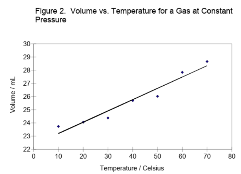
Figure 2 shows example student data for the volume of a sample of gas as a function of temperature. Both the volume (y) and temperature (x) measurements were subject to random errors, but those in the volume greatly exceeded those in the temperature. Hence, the points deviate from a straight line due mainly to the random errors in the volumes. The best line through the data points should then minimize the magnitude of the vertical (y) deviations between the experimental points and the line. Since these deviations are positive and negative, the squares of the deviations are minimized (hence, the name least squares).
Minimizing the sum of the squares of the deviations corresponds to assuming that the observed set of volumes is the most probable set. The probability of observing a particular volume, \(\ce{V_{i}}\), for some temperature, \(\ce{t_{i}}\), is given by a Gaussian curve with the true volume \(\ce{(\mu_{v})}\) given by equation (9). The probability of obtaining the observed set of volumes is given by the product of these Gaussian curves. Maximizing this probability, so that the observed volumes are the most probable set, is equivalent to minimizing the sum of the squares of the vertical deviations. The minimization is accomplished using differential calculus, and yields equations for the slope and intercept of the best line in terms of all of the data points (all of the pairs \(\ce{V_{i}}\) and \(\ce{t_{i}}\) or, more generally, \(\ce{y_{i}}\) and \(\ce{x_{i}}\)). The resulting equations for the slope and intercept and for the standard deviations in these quantities are given in a variety of texts.* They will not be repeated here, since in this course you will use the built-in functions of a microcomputer spreadsheet to perform least squares analyses.
The line shown in Figure 2 results from a least squares fit to the experimental data. The parameters of this best-fit line and their standard deviations, obtained using a spreadsheet, are given below.
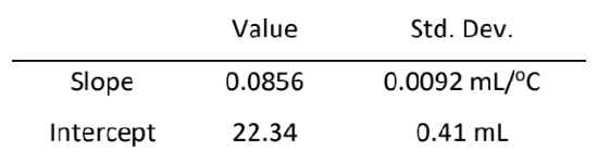
The sum of the vertical deviations, including their signs, of the experimental data points from this line equals zero, which is what one would intuitively attempt to accomplish in visually drawing the line. The sum of the deviations will always be zero for the best line, just as the sum of the deviations from an average or mean will always be zero.
The best-fit parameters yield \( \ce{ t_{0} = - (\frac{22.34}{0.0856}) = -261 }\)°C. We can obtain the uncertainty in \( \ce{t_{0}}\) by propagating the uncertainties in the slope and intercept using the formula given earlier for division involving independent variables. This is only approximately correct in the present case since the slope and intercept are correlated, and not independent. The full treatment for correlated variables, however, is beyond the scope of this introduction. The earlier formula, equation (7), gives
\( \ce{ St_{0} = 261[(\frac{0.0092}{0.0856})^{2} + (\frac{0.41}{22.34})^{2}]^{1/2} }\)
\(\ce{ 261(0.109) = 28 }\)°C
Hence, the extrapolated value of t0 agrees with the expected value within one (approximate) standard deviation.
We will now confess the truth about the "student data" in Figure 2. This was generated by adding a purely random number between -0.5 and +0.5 mL to the volume calculated for each temperature from equation (9) with \(\ce{ n = 1.0 x 10^{-3} }\) moles, \( \ce{ P = 1.0 }\) atm, and \( \ce{ R = 82.06 }\) \(\ce { \frac{mL*atm}{mol*K}} \). Hence, the expected slope is \( \ce{ (\frac{nR}{P}) = 0.08206 \frac{mL}{°C} }\), and the expected intercept is \( \ce{ (\frac{nR}{P})(273.15) = 22.414 }\) mL. The corresponding parameters derived by the least squares analysis differ from the expected values because of the random errors added to the volume. However, the derived parameters do agree with the expected or true values within one standard deviation.
Questions (Only for students who did not take 4A)
1. Multiple determinations of the percent by mass of iron in an unknown ore yield 15.31, 15.30, 15.26, 15.28 and 15.29%. Calculate:
(a) The mean percent by mass of iron;
(b) The sample standard deviation;
(c) The standard deviation of the mean;
(d) and the 95% CL of the mean.
2. For each of the following data sets, determine whether any measurement should be rejected at the 90% confidence level using the Q test.
(a) 2.8, 2.7, 2.5, 2.9, 2.6, 3.0, 2.6
(b) 97.13, 97.10, 97.20, 97.35, 97.10, 97.15
(c) 0.134, 0.120, 0.109, 0.124, 0.131, 0.119
3. A chemist determines the number of moles, n, of some gas from measurements of the pressure, P, volume, V, and temperature, T, of the gas, using the ideal gas equation of state, as \(\ce{n = \frac{PV}{RT}}\). The results of the measurements, with the estimated standard deviations in parentheses, are \(\ce{P = 0.235 (0.005)}\) atm, \(\ce{V = 1.22 (0.03)}\) L, and \(\ce{T = 310 (2)}\) K. The constant R equals \(\ce{0.08206 \frac{L*atm}{mol*K}}\). Calculate n and its estimated standard deviation.
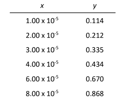
4. Use the method of least squares to find the slope, m, intercept, b, and the respective standard deviations of the best straight line, \(\ce{ y = mx + b}\), for representing the following data