
5: Measurement of Planck's Constant (Experiment)
- Page ID
- 416884
\( \newcommand{\vecs}[1]{\overset { \scriptstyle \rightharpoonup} {\mathbf{#1}} } \)
\( \newcommand{\vecd}[1]{\overset{-\!-\!\rightharpoonup}{\vphantom{a}\smash {#1}}} \)
\( \newcommand{\dsum}{\displaystyle\sum\limits} \)
\( \newcommand{\dint}{\displaystyle\int\limits} \)
\( \newcommand{\dlim}{\displaystyle\lim\limits} \)
\( \newcommand{\id}{\mathrm{id}}\) \( \newcommand{\Span}{\mathrm{span}}\)
( \newcommand{\kernel}{\mathrm{null}\,}\) \( \newcommand{\range}{\mathrm{range}\,}\)
\( \newcommand{\RealPart}{\mathrm{Re}}\) \( \newcommand{\ImaginaryPart}{\mathrm{Im}}\)
\( \newcommand{\Argument}{\mathrm{Arg}}\) \( \newcommand{\norm}[1]{\| #1 \|}\)
\( \newcommand{\inner}[2]{\langle #1, #2 \rangle}\)
\( \newcommand{\Span}{\mathrm{span}}\)
\( \newcommand{\id}{\mathrm{id}}\)
\( \newcommand{\Span}{\mathrm{span}}\)
\( \newcommand{\kernel}{\mathrm{null}\,}\)
\( \newcommand{\range}{\mathrm{range}\,}\)
\( \newcommand{\RealPart}{\mathrm{Re}}\)
\( \newcommand{\ImaginaryPart}{\mathrm{Im}}\)
\( \newcommand{\Argument}{\mathrm{Arg}}\)
\( \newcommand{\norm}[1]{\| #1 \|}\)
\( \newcommand{\inner}[2]{\langle #1, #2 \rangle}\)
\( \newcommand{\Span}{\mathrm{span}}\) \( \newcommand{\AA}{\unicode[.8,0]{x212B}}\)
\( \newcommand{\vectorA}[1]{\vec{#1}} % arrow\)
\( \newcommand{\vectorAt}[1]{\vec{\text{#1}}} % arrow\)
\( \newcommand{\vectorB}[1]{\overset { \scriptstyle \rightharpoonup} {\mathbf{#1}} } \)
\( \newcommand{\vectorC}[1]{\textbf{#1}} \)
\( \newcommand{\vectorD}[1]{\overrightarrow{#1}} \)
\( \newcommand{\vectorDt}[1]{\overrightarrow{\text{#1}}} \)
\( \newcommand{\vectE}[1]{\overset{-\!-\!\rightharpoonup}{\vphantom{a}\smash{\mathbf {#1}}}} \)
\( \newcommand{\vecs}[1]{\overset { \scriptstyle \rightharpoonup} {\mathbf{#1}} } \)
\(\newcommand{\longvect}{\overrightarrow}\)
\( \newcommand{\vecd}[1]{\overset{-\!-\!\rightharpoonup}{\vphantom{a}\smash {#1}}} \)
\(\newcommand{\avec}{\mathbf a}\) \(\newcommand{\bvec}{\mathbf b}\) \(\newcommand{\cvec}{\mathbf c}\) \(\newcommand{\dvec}{\mathbf d}\) \(\newcommand{\dtil}{\widetilde{\mathbf d}}\) \(\newcommand{\evec}{\mathbf e}\) \(\newcommand{\fvec}{\mathbf f}\) \(\newcommand{\nvec}{\mathbf n}\) \(\newcommand{\pvec}{\mathbf p}\) \(\newcommand{\qvec}{\mathbf q}\) \(\newcommand{\svec}{\mathbf s}\) \(\newcommand{\tvec}{\mathbf t}\) \(\newcommand{\uvec}{\mathbf u}\) \(\newcommand{\vvec}{\mathbf v}\) \(\newcommand{\wvec}{\mathbf w}\) \(\newcommand{\xvec}{\mathbf x}\) \(\newcommand{\yvec}{\mathbf y}\) \(\newcommand{\zvec}{\mathbf z}\) \(\newcommand{\rvec}{\mathbf r}\) \(\newcommand{\mvec}{\mathbf m}\) \(\newcommand{\zerovec}{\mathbf 0}\) \(\newcommand{\onevec}{\mathbf 1}\) \(\newcommand{\real}{\mathbb R}\) \(\newcommand{\twovec}[2]{\left[\begin{array}{r}#1 \\ #2 \end{array}\right]}\) \(\newcommand{\ctwovec}[2]{\left[\begin{array}{c}#1 \\ #2 \end{array}\right]}\) \(\newcommand{\threevec}[3]{\left[\begin{array}{r}#1 \\ #2 \\ #3 \end{array}\right]}\) \(\newcommand{\cthreevec}[3]{\left[\begin{array}{c}#1 \\ #2 \\ #3 \end{array}\right]}\) \(\newcommand{\fourvec}[4]{\left[\begin{array}{r}#1 \\ #2 \\ #3 \\ #4 \end{array}\right]}\) \(\newcommand{\cfourvec}[4]{\left[\begin{array}{c}#1 \\ #2 \\ #3 \\ #4 \end{array}\right]}\) \(\newcommand{\fivevec}[5]{\left[\begin{array}{r}#1 \\ #2 \\ #3 \\ #4 \\ #5 \\ \end{array}\right]}\) \(\newcommand{\cfivevec}[5]{\left[\begin{array}{c}#1 \\ #2 \\ #3 \\ #4 \\ #5 \\ \end{array}\right]}\) \(\newcommand{\mattwo}[4]{\left[\begin{array}{rr}#1 \amp #2 \\ #3 \amp #4 \\ \end{array}\right]}\) \(\newcommand{\laspan}[1]{\text{Span}\{#1\}}\) \(\newcommand{\bcal}{\cal B}\) \(\newcommand{\ccal}{\cal C}\) \(\newcommand{\scal}{\cal S}\) \(\newcommand{\wcal}{\cal W}\) \(\newcommand{\ecal}{\cal E}\) \(\newcommand{\coords}[2]{\left\{#1\right\}_{#2}}\) \(\newcommand{\gray}[1]{\color{gray}{#1}}\) \(\newcommand{\lgray}[1]{\color{lightgray}{#1}}\) \(\newcommand{\rank}{\operatorname{rank}}\) \(\newcommand{\row}{\text{Row}}\) \(\newcommand{\col}{\text{Col}}\) \(\renewcommand{\row}{\text{Row}}\) \(\newcommand{\nul}{\text{Nul}}\) \(\newcommand{\var}{\text{Var}}\) \(\newcommand{\corr}{\text{corr}}\) \(\newcommand{\len}[1]{\left|#1\right|}\) \(\newcommand{\bbar}{\overline{\bvec}}\) \(\newcommand{\bhat}{\widehat{\bvec}}\) \(\newcommand{\bperp}{\bvec^\perp}\) \(\newcommand{\xhat}{\widehat{\xvec}}\) \(\newcommand{\vhat}{\widehat{\vvec}}\) \(\newcommand{\uhat}{\widehat{\uvec}}\) \(\newcommand{\what}{\widehat{\wvec}}\) \(\newcommand{\Sighat}{\widehat{\Sigma}}\) \(\newcommand{\lt}{<}\) \(\newcommand{\gt}{>}\) \(\newcommand{\amp}{&}\) \(\definecolor{fillinmathshade}{gray}{0.9}\)Hazard Overview
Chemical Hazards
N/A
Mechanical Hazards
Electrical hazard (power supply)
Dispensary Provided Items
- LED apparatus
- Oscilloscope
Introduction
Planck's constant is one of the fundamental quantities of physics, and the chemical and physical laws of nature are dependent on its magnitude. In this experiment, you will measure Planck's constant by investigating the current-voltage characteristics of and the colors emitted by a series of light-emitting diodes.
Light-emitting diodes (LEDs) are widely used as components in various consumer products. For example, cell phone displays, computer monitors, TVs, and modern lighting all use visible wavelength LEDs. The lighthouse base station used by some VR headsets uses LEDs that emit at wavelengths beyond the visible spectrum (in the infrared). Most commercial LEDs are based on GaAs and GaP, so-called III-V semiconductors, since they are made up of elements from groups III and V of the periodic table. Crystals with the general composition \( \ce{GaAs_{1-x}P_x} \), where x varies between 0 and 1, can be produced. The crystals are doped purposefully with small amounts of different impurities in adjacent regions to form a p-n junction or diode. The resulting doped crystals efficiently emit light when a voltage is applied across the junction. The color of the emitted light depends on the exact value of x. For example, the light of wavelength around 950 nm (infrared) is emitted for x = 0, and around 560 nm (green) for x = 1. LEDs that emit at shorter wavelengths are based on \( \ce{SiC} \). The technology to produce these well-defined, doped crystals under industrial conditions became available only in the late 1960s, and their use in a variety of consumer products has spread rapidly since then.
The operation of an LED depends on the quantized energy levels of the crystal. Let's consider a hypothetical pure crystal containing a large number (roughly Avogadro's number) of identical entities (atoms or molecules). The energy levels (states) of each entity comprising the crystal are identical if the entities are not interacting. Hence, the number of states with a particular energy, or the degeneracy, for the collection of non-interacting entities is very large. Interactions among the entities in the crystal cause these states to have different energies, leading to a spread of energies or an energy band. The details of the band will depend on the electronic structure of the atoms or molecules comprising the crystal and the interactions among these in the crystal. In a pure semiconductor, two bands result from the interaction of the valence orbitals, each containing half the total number of states. The lower band is called the valence band, and the upper one is called the conduction band. The energy difference between the bottom of the conduction band and the top of the valence band is called the band gap, \( {E_g} \). The electrons in a pure semiconductor cannot assume energies within this forbidden gap. The process is diagrammed in Figure \(\PageIndex{1}\).

The valence band of a pure semiconductor is typically filled, meaning that it contains just the number of electrons that are required to completely fill with opposite spins all of the levels in the band. Its conduction band is essentially empty. In the p region of a diode, the impurity dopant has removed electrons from the valence band, causing vacancies or holes to be produced in the valence band, whereas in the n region, the impurity has added electrons to the conduction band. A barrier exists, however, for the movement of an electron (or a hole) between the n and p regions of the diode. Depending on the particular diode, this barrier is equal to, or slightly lower in energy than, the band gap. If an external voltage that counteracts the barrier is applied across the junction, electrons will flow (be injected) across the junction boundary from the n to the p region.

Figure \(\PageIndex{2}\) shows the expected current-voltage behavior of an ideal diode. For low applied voltages, there is not enough energy to overcome the barrier between the n and p regions. Hence, no current flows through the diode. When the voltage corresponding to the band gap is reached, the current begins to flow. At even higher voltages, the current increases in proportion to the number of electrons injected into the p region. The behavior shown in Figure \(\PageIndex{2}\) is reminiscent of the photoelectric effect, except that here the current instead of the kinetic energy of the electrons is measured, and the energy is supplied by an applied voltage rather than light. The energy acquired by the electron from the applied voltage is given by eV (read as electron volt), where e is the electron charge (1.6021773 \( \times 10^{-19} \) C) and V is the applied voltage. Since 1 V = 1 J/C, an electron subjected to one volt acquires an energy of 1 eV = 1.6021773 \( \times 10^{-19} \) J = 96.48531 kJ/mol. Hence, the voltage at which current begins to flow for a particular diode numerically equals the band gap of the diode in eV.
What happens to the electrons injected into the p region by the applied voltage? These electrons will lose energy by falling into the holes in the lower energy valence band. The released energy appears as heat in a conventional diode. However, in an LED the energy released by some of the electrons falling into the valence band appears as light energy. The color or wavelength of the emitted light depends on the band gap of the material through the Planck-Einstein relation, given by:
\[ E_g = h\nu = \frac{hc}{\lambda} \]
where \( h \) is Planck's constant, \( \nu \) is the frequency of the light, \( \lambda \) is the wavelength of light, and \( c = 299792458 \space m/s \), the speed of light in a vacuum. In SI units, the energy is in \( J \), the frequency is in \( s^{-1} \) or Hz, the wavelength is in m, and h is in \( J \cdot s \). Note that as the applied voltage is increased from zero, the emission of light appears simultaneously with the current flow, since both the light emission and the current flow depend on the injection of electrons into the junction region of the diode. The two phenomena are linked. Plotting the band gap, \( {E_g} \), against the inverse wavelength, \( 1/\lambda \), of the emitted light for a series of LEDs should yield a straight line with an intercept of zero and a slope equal to \( hc \).
In the present experiment, you will measure the band gaps for a series of LEDs from their current-voltage characteristics. You will also determine the peak wavelengths of their emissions using a simple spectroscope and fit your data to estimate Planck's constant.
Operation of Lab Equipment
Operation of a Spectroscope
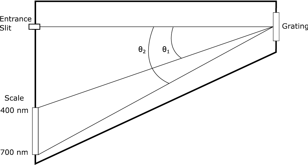
A simple spectroscope uses a grating to disperse light into its various wavelengths. A transmission grating consists of a series of parallel grooves on a flat transparent surface. When light is incident on the grating, each groove acts as a separate source of light waves for the transmitted light, creating interference in the light waves. For constructive interference, the transmitted waves must be in phase with their maxima and minima overlapping in space. Constructive interference occurs when
\[ n\lambda = d \sin\theta \]
where \( n \) is an integer, \( \lambda \) is the wavelength of the light wave, and \( d \) is the spacing between the grooves of the grating. The grating acts to disperse the light into its various wavelengths since each wavelength has its maximum intensity at a particular angle, \( \theta \), for constant \( d \) and a given \( n \). When \( n \) = 1, the image of the diffracted light is called the first-order image.
A schematic of a spectroscope is shown in Figure \(\PageIndex{3}\) Light enters the spectroscope through a slit and exits through a transmission grating to the eye of the viewer. Since the transmitted light undergoes interference, a virtual image of the slit occurs at an angle \( \theta \), dependent on the grating spacing and the wavelength of the light. A scale is attached to the spectroscope that allows the wavelength of the light to be read from the position of the first-order image. The width of the image for monochromatic light depends on the width of the slit. The larger the dimensions of the spectroscope and the smaller the grating spacing, the more accurately the position of the image can be determined for a fixed slit width. Research-grade spectrometers use reflection gratings and photoelectric detection of real images. These instruments can exceed several meters.
Experimental Procedure
You will study six different LEDs in this experiment. The wavelengths of their emitted light will be measured using a simple spectroscope for the five LEDs that emit in the visible region of the spectrum, and you will use an oscilloscope to measure their band gap characteristics. The procedure is outlined below.
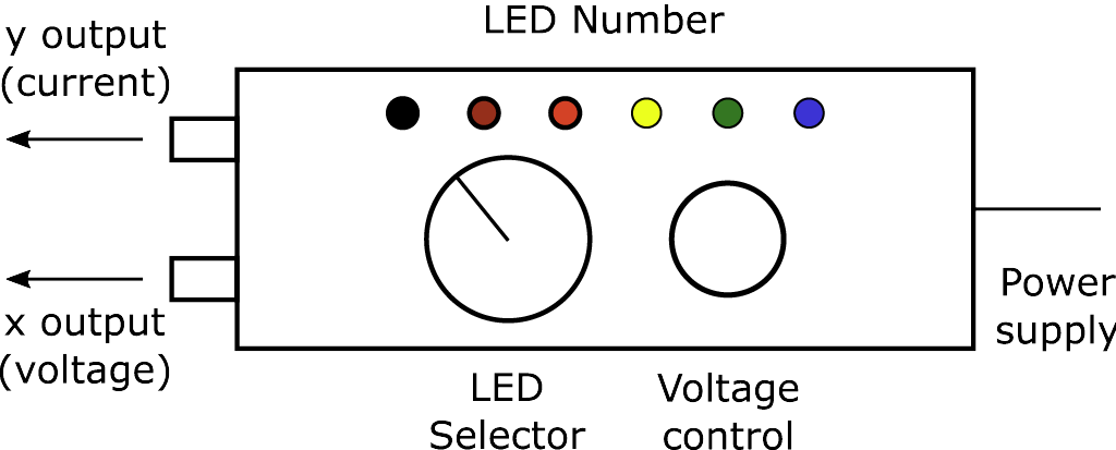
Figure \(\PageIndex{4}\) shows a sketch of the apparatus that houses the LEDs with its attached power supply. An individual LED is chosen by the selector switch. Position 1 on the switch corresponds to LED 1 (blue) and position 6 to LED 6 (IR). Intermediate positions on the switch select the other LEDs in order of their emission wavelengths. Position 0 disconnects the LEDs from the circuit. The other control adjusts the maximum applied voltage and, thereby, the intensity of the light emitted by the chosen LED. The two BNC connectors on the apparatus provide two output voltages. The output labeled X gives the voltage that is applied across the LED. The output labeled Y gives a voltage that is proportional to the current through the LED (the current in amps is given by 0.01 times the Y output in volts).
Ensure the power supply is plugged into the line voltage. Do not turn off the power supply throughout the experiment. Switch the selector to position 1 and adjust the voltage control from minimum (fully counterclockwise) to maximum (fully clockwise) while observing the blue LED. Similarly, examine the LEDs corresponding to positions 2 to 5, recording the visual color of each of the LEDs. Then, using a hand-held spectroscope, view in turn each of the lighted LEDs to determine the wavelength of their emitted light. Record the peak wavelength (the wavelength of maximum intensity) for each of the five LEDs 1 to 5, estimating to 5 nm. The peak wavelength for LED 6 is in the infrared at 950 nm, which is beyond the visible range.
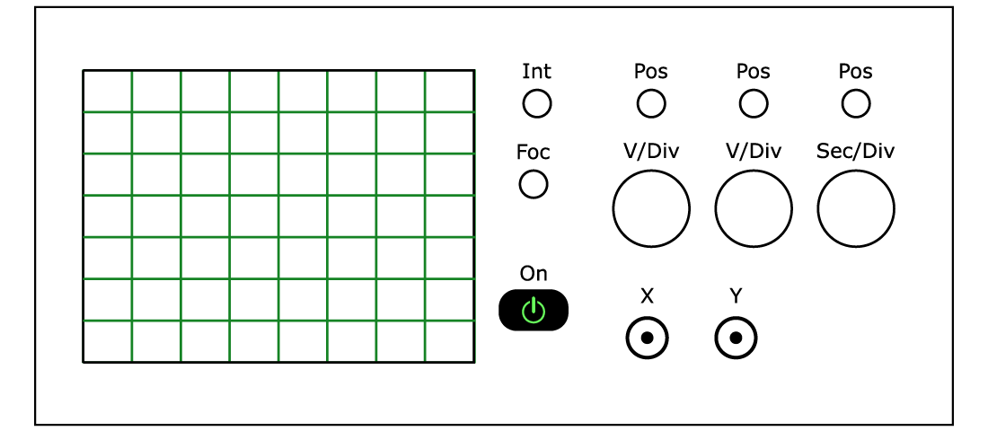
You will next use an oscilloscope to deduce the band gaps of the LEDs. A schematic of an oscilloscope is shown in Figure \(\PageIndex{5}\) with its inputs and major controls identified. The oscilloscope has two inputs that are labeled CH 1 or X and CH 2 or Y (CH stands for channel). When the Sec/Div switch is set to X-Y, voltages at the X and Y inputs will cause the oscilloscope to show a Y (vertical) versus X (horizontal) trace on its display. The volts per division along the Y and X axes are set by the Volts/Div switch for the corresponding axis. The position on the display corresponding to zero volts for the Y input is adjusted by the Position control above the V/Div switch for the Y input. The position for the X input is adjusted by the control above the Sec/Div switch, not by the corresponding control for the X input. The intensity of the trace and its focus are adjusted by the controls adjacent to the display above the power-on switch. All controls you need for this experiment are highlighted on the scopes you will use.
Set the oscilloscope Sec/Div switch to X-Y. Ground the X and Y inputs by sliding the switches labeled AC-GND-DC (located directly above the inputs) to GND. Then, move the position of the spot on the display to the intersection of the center horizontal graticule and the first vertical graticule from the left of the display. This sets the origin or the position of zero volts on the display. Slide the switches to DC to make measurements.
Set the selector switch of the LED apparatus to position 0, adjust its voltage control to minimum, and connect its X and Y outputs to the X and Y inputs, respectively, of the oscilloscope with electrical cables. Then, select LED 1 and slowly turn the voltage control to its maximum on the LED apparatus, while observing the display on the oscilloscope. You should obtain a trace on the display similar to one of the traces in Figure \(\PageIndex{2}\). The trace should be a horizontal line from zero volts to a voltage slightly less than the band gap, a transitional curving portion just before the band gap, and a positively sloping line at higher voltages. Note that the LED lights at the voltage corresponding to the onset of the positively sloping portion of the trace, namely when current flows through the diode. Visually extrapolate the linear, sloping portion of the trace to intersect the extension of the horizontal portion in order to estimate the voltage corresponding to the band gap of the LED. The setting of the V/Div switch for CH 1 or X gives the volts per line along the horizontal axis (the minor ticks along the middle graticules are at 0.2 divisions). Similarly, estimate the band gaps of the other LEDs, including the LED at position 6, whose emission is in the infrared. The band gaps are in the range of 1-3 eV, so the horizontal sensitivity should be in the range of 0.2-0.5 volts per division, in order that the origin (zero volts) and the onset of the sloping portion are simultaneously visible in the display. You should use the most sensitive setting possible for each LED, to get the best estimate of its band gap.
You may have to adjust the volts/div when switching to a different LED to be able to accurately measure the band gap.
The vertical sensitivity should be adjusted for ease in the extrapolation of the sloping line to the horizontal axis (approximately 0.2-1.0 volts per division). Before you record your estimate for the band gap, it is prudent to again ground the X and Y inputs to check that the position of zero volts has not moved.
Lab Report
Be sure to calculate the following for your lab report:
- Graph the band gaps in eV for the six LEDs against the inverse of their peak wavelengths in nm. Fit the data to the equation for a straight line, and calculate Planck's constant in J s from the slope. Note that the y-intercept is 0, if it is not, you should force the intercept through zero.
- Report your graph, your best estimate for Planck's constant in J s, % error in Planck's constant, and its standard deviation in J s.
Also, include the answers to the following questions in your lab report.
- Compare your result for Planck's constant with the accepted value of 6.626076 \( \times 10^{-34} \) J s. Discuss possible reasons for any disagreement.
- A LED emits light with a wavelength of 940\( \pm \)5 nm. What is the band gap and its error in eV?
- Light with a wavelength of 800 nm is incident on a transmission grating that has 1200 grooves per mm. Calculate the diffraction angle \( \theta \) (see Figure \(\PageIndex{3}\)) for the first order image.
- A potential problem when using diffraction gratings is that the images for different wavelengths can occur at the same diffraction angle in different orders. What other wavelengths, and in what order, have images that occur at the same diffraction angle as that for 800 nm light in the first order?
Data Table
| LED Number | Visual Color | Wavelength (nm) | Band Gap (eV) |
|---|---|---|---|
| 1 | |||
| 2 | |||
| 3 | |||
| 4 | |||
| 5 | |||
| 6 | IR | 950 |
| Planck's Constant (J s) | |||
| Standard Deviation (J s) | |||