
3.2: Lagrange's Method of Undetermined Multipliers
- Page ID
- 206317

\( \newcommand{\vecs}[1]{\overset { \scriptstyle \rightharpoonup} {\mathbf{#1}} } \)
\( \newcommand{\vecd}[1]{\overset{-\!-\!\rightharpoonup}{\vphantom{a}\smash {#1}}} \)
\( \newcommand{\id}{\mathrm{id}}\) \( \newcommand{\Span}{\mathrm{span}}\)
( \newcommand{\kernel}{\mathrm{null}\,}\) \( \newcommand{\range}{\mathrm{range}\,}\)
\( \newcommand{\RealPart}{\mathrm{Re}}\) \( \newcommand{\ImaginaryPart}{\mathrm{Im}}\)
\( \newcommand{\Argument}{\mathrm{Arg}}\) \( \newcommand{\norm}[1]{\| #1 \|}\)
\( \newcommand{\inner}[2]{\langle #1, #2 \rangle}\)
\( \newcommand{\Span}{\mathrm{span}}\)
\( \newcommand{\id}{\mathrm{id}}\)
\( \newcommand{\Span}{\mathrm{span}}\)
\( \newcommand{\kernel}{\mathrm{null}\,}\)
\( \newcommand{\range}{\mathrm{range}\,}\)
\( \newcommand{\RealPart}{\mathrm{Re}}\)
\( \newcommand{\ImaginaryPart}{\mathrm{Im}}\)
\( \newcommand{\Argument}{\mathrm{Arg}}\)
\( \newcommand{\norm}[1]{\| #1 \|}\)
\( \newcommand{\inner}[2]{\langle #1, #2 \rangle}\)
\( \newcommand{\Span}{\mathrm{span}}\) \( \newcommand{\AA}{\unicode[.8,0]{x212B}}\)
\( \newcommand{\vectorA}[1]{\vec{#1}} % arrow\)
\( \newcommand{\vectorAt}[1]{\vec{\text{#1}}} % arrow\)
\( \newcommand{\vectorB}[1]{\overset { \scriptstyle \rightharpoonup} {\mathbf{#1}} } \)
\( \newcommand{\vectorC}[1]{\textbf{#1}} \)
\( \newcommand{\vectorD}[1]{\overrightarrow{#1}} \)
\( \newcommand{\vectorDt}[1]{\overrightarrow{\text{#1}}} \)
\( \newcommand{\vectE}[1]{\overset{-\!-\!\rightharpoonup}{\vphantom{a}\smash{\mathbf {#1}}}} \)
\( \newcommand{\vecs}[1]{\overset { \scriptstyle \rightharpoonup} {\mathbf{#1}} } \)
\( \newcommand{\vecd}[1]{\overset{-\!-\!\rightharpoonup}{\vphantom{a}\smash {#1}}} \)
\(\newcommand{\avec}{\mathbf a}\) \(\newcommand{\bvec}{\mathbf b}\) \(\newcommand{\cvec}{\mathbf c}\) \(\newcommand{\dvec}{\mathbf d}\) \(\newcommand{\dtil}{\widetilde{\mathbf d}}\) \(\newcommand{\evec}{\mathbf e}\) \(\newcommand{\fvec}{\mathbf f}\) \(\newcommand{\nvec}{\mathbf n}\) \(\newcommand{\pvec}{\mathbf p}\) \(\newcommand{\qvec}{\mathbf q}\) \(\newcommand{\svec}{\mathbf s}\) \(\newcommand{\tvec}{\mathbf t}\) \(\newcommand{\uvec}{\mathbf u}\) \(\newcommand{\vvec}{\mathbf v}\) \(\newcommand{\wvec}{\mathbf w}\) \(\newcommand{\xvec}{\mathbf x}\) \(\newcommand{\yvec}{\mathbf y}\) \(\newcommand{\zvec}{\mathbf z}\) \(\newcommand{\rvec}{\mathbf r}\) \(\newcommand{\mvec}{\mathbf m}\) \(\newcommand{\zerovec}{\mathbf 0}\) \(\newcommand{\onevec}{\mathbf 1}\) \(\newcommand{\real}{\mathbb R}\) \(\newcommand{\twovec}[2]{\left[\begin{array}{r}#1 \\ #2 \end{array}\right]}\) \(\newcommand{\ctwovec}[2]{\left[\begin{array}{c}#1 \\ #2 \end{array}\right]}\) \(\newcommand{\threevec}[3]{\left[\begin{array}{r}#1 \\ #2 \\ #3 \end{array}\right]}\) \(\newcommand{\cthreevec}[3]{\left[\begin{array}{c}#1 \\ #2 \\ #3 \end{array}\right]}\) \(\newcommand{\fourvec}[4]{\left[\begin{array}{r}#1 \\ #2 \\ #3 \\ #4 \end{array}\right]}\) \(\newcommand{\cfourvec}[4]{\left[\begin{array}{c}#1 \\ #2 \\ #3 \\ #4 \end{array}\right]}\) \(\newcommand{\fivevec}[5]{\left[\begin{array}{r}#1 \\ #2 \\ #3 \\ #4 \\ #5 \\ \end{array}\right]}\) \(\newcommand{\cfivevec}[5]{\left[\begin{array}{c}#1 \\ #2 \\ #3 \\ #4 \\ #5 \\ \end{array}\right]}\) \(\newcommand{\mattwo}[4]{\left[\begin{array}{rr}#1 \amp #2 \\ #3 \amp #4 \\ \end{array}\right]}\) \(\newcommand{\laspan}[1]{\text{Span}\{#1\}}\) \(\newcommand{\bcal}{\cal B}\) \(\newcommand{\ccal}{\cal C}\) \(\newcommand{\scal}{\cal S}\) \(\newcommand{\wcal}{\cal W}\) \(\newcommand{\ecal}{\cal E}\) \(\newcommand{\coords}[2]{\left\{#1\right\}_{#2}}\) \(\newcommand{\gray}[1]{\color{gray}{#1}}\) \(\newcommand{\lgray}[1]{\color{lightgray}{#1}}\) \(\newcommand{\rank}{\operatorname{rank}}\) \(\newcommand{\row}{\text{Row}}\) \(\newcommand{\col}{\text{Col}}\) \(\renewcommand{\row}{\text{Row}}\) \(\newcommand{\nul}{\text{Nul}}\) \(\newcommand{\var}{\text{Var}}\) \(\newcommand{\corr}{\text{corr}}\) \(\newcommand{\len}[1]{\left|#1\right|}\) \(\newcommand{\bbar}{\overline{\bvec}}\) \(\newcommand{\bhat}{\widehat{\bvec}}\) \(\newcommand{\bperp}{\bvec^\perp}\) \(\newcommand{\xhat}{\widehat{\xvec}}\) \(\newcommand{\vhat}{\widehat{\vvec}}\) \(\newcommand{\uhat}{\widehat{\uvec}}\) \(\newcommand{\what}{\widehat{\wvec}}\) \(\newcommand{\Sighat}{\widehat{\Sigma}}\) \(\newcommand{\lt}{<}\) \(\newcommand{\gt}{>}\) \(\newcommand{\amp}{&}\) \(\definecolor{fillinmathshade}{gray}{0.9}\)Lagrange’s method of undetermined multipliers is a method for finding the minimum or maximum value of a function subject to one or more constraints. A simple example serves to clarify the general problem. Consider the function
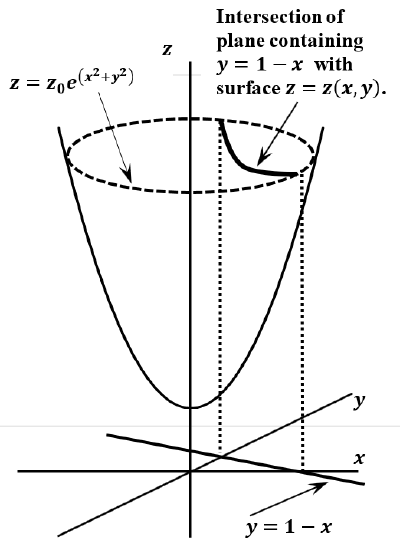
\[z=z_0\ \mathrm{exp}\left(x^2+y^2\right)\nonumber \]
where \(z_0\) is a constant. This function is a surface of revolution, which is tangent to the plane \(z=z_0\) at \(\left(0,0,z_0\right)\). The point of tangency is the minimum value of \(z\). At any other point in the \(xy\)-plane, \(z\left(x,y\right)\) is greater than \(z_0\). If either \(x\) or \(y\) becomes arbitrarily large, \(z\) does also. If we project a contour of constant \(z\) onto the \(xy\)-plane, the projection is a circle of radius
\[r=\left(x^2+y^2\right)^{1/2}. \nonumber \]
Suppose that we introduce an additional condition; we require \(y=1-x\). Then we ask for the smallest value of \(z\) consistent with this constraint. In the \(xy\)-plane the constraint is a line of slope \(-1\) and intercept \(1\). A plane that includes this line and is parallel to the \(z\)-axis intersects the function \(z\). As sketched in Figure 1, this intersection is a curve. Far away from the origin, the value of \(z\) at which the intersection occurs is large. Nearer the origin, the value of \(z\) is smaller, and there is some \(\left(x,y\right)\) at which it is a minimum. Our objective is to find this minimum.
There is a straightforward solution of this problem; we can substitute the constraint equation for \(y\) into the equation for\(\ z\), making \(z\) a function of only one variable, \(x\). We have
\[ \begin{align*} z&=z_0\ \mathrm{exp} \left(x^2+{\left(1-x\right)}^2\right) \\[4pt] &=z_0\ \mathrm{exp} \left(2x^2-2x+1\right)\end{align*} \nonumber \]
To find the minimum, we equate the derivative to zero, giving
\[0=\frac{dz}{dx}=\left(4x-2\right)z_0\ \mathrm{exp} \left(2x^2-2x+1\right)\nonumber \]
so that the minimum occurs at \(x={1}/{2}\), y\(={1}/{2}\), and
\[z=z_0\ \mathrm{exp}\left({1}/{2}\right)\nonumber \]
Solving such problems by elimination of variables can become difficult. Lagrange’s method of undetermined multipliers is a general method, which is usually easy to apply and which is readily extended to cases in which there are multiple constraints. We can see how Lagrange’s method arises by thinking further about our particular example. We can imagine that we “walk” along the constraint line in the \(xy\)-plane and measure the \(z\) that is directly overhead as we progress. The problem is to find the minimum value of \(z\) that we encounter as we proceed along the line. This perspective highlights the central feature of the problem: While it is formally a problem in three dimensions (\(x\), \(y\), and \(z\)), the introduction of the constraint makes it a two-dimensional problem. We can think of one dimension as a displacement along the line \(y=1-x\), from some arbitrary starting point on the line. The other dimension is the perpendicular distance from the \(xy\)-plane to the intersection with the surface \(z\).
The relevant part of the \(xy\)-plane is just the one-dimensional constraint line. We can recognize this by parameterizing the line. Let \(t\) measure location on the line relative to some initial point at which \(t\ =\ 0\). Then we have \(x=x\left(t\right)\) and \(y=y\left(t\right)\) and
\[z\left(x,y\right)=z\left(x\left(t\right),y\left(t\right)\right)=z\left(t\right).\nonumber \]
The point we seek is the one at which \({dz}/{dt}=0\).
Now let us examine a somewhat more general problem. We want a general way to find the values \(\left(x,y\right)\) that minimize (or maximize) a function \(h=h\left(x,y\right)\) subject to a constraint of the form \(c=g\left(x,y\right)\), where \(c\) is a constant. As in our example, this constraint requires a solution in which \(\left(x,y\right)\) are on a particular line. If we parameterize this problem, we have
\[h=h\left(x,y\right)=h\left(x\left(t\right),y\left(t\right)\right)=h\left(t\right)\nonumber \]
and
\[c=g\left(x,y\right)=g\left(x\left(t\right),y\left(t\right)\right)=g\left(t\right)\nonumber \]
Because \(c\) is a constant, \({dc}/{dt}={dg}/{dt}=0\). The solution we seek is the point at which \(h\) is an extremum. At this point, \({dh}/{dt}=0\). Therefore, at the point we seek, we have
\[\frac{dh}{dt}={\left(\frac{\partial h}{\partial x}\right)}_y\frac{dx}{dt}+{\left(\frac{\partial h}{\partial y}\right)}_x\frac{dy}{dt}=0\nonumber \] and \[\frac{dg}{dt}={\left(\frac{\partial g}{\partial x}\right)}_y\frac{dx}{dt}+{\left(\frac{\partial g}{\partial y}\right)}_x\frac{dy}{dt}=0\nonumber \]
We can multiply either of these equations by any factor, and the product will be zero. We multiply \({dg}/{dt}\) by \(\lambda\) (where \(\lambda \neq 0\)) and subtract the result from \({dh}/{dt}\). Then, at the point we seek,
\[0=\frac{dh}{dt}-\lambda \frac{dg}{dt}={\left(\frac{\partial h}{\partial x}-\lambda \frac{\partial g}{\partial x}\right)}_y\frac{dx}{dt}+{\left(\frac{\partial h}{\partial y}-\lambda \frac{\partial g}{\partial y}\right)}_x\frac{dy}{dt}\nonumber \]
Since we can choose \(x\left(t\right)\) and \(y\left(t\right)\) any way we please, we can insure that \({dx}/{dt}\neq 0\) and \({dy}/{dt}\neq 0\) at the solution point. If we do so, the terms in parentheses must be zero at the solution point.
Conversely, setting
\[{\left(\frac{\partial h}{\partial x}-\lambda \frac{\partial g}{\partial x}\right)}_y=0\nonumber \] and \[{\left(\frac{\partial h}{\partial y}-\lambda \frac{\partial g}{\partial y}\right)}_x=0\nonumber \]
is sufficient to insure that
\[\frac{dh}{dt}=\lambda \frac{dg}{dt}\nonumber \]
Since \({dg}/{dt}=0\), these conditions insure that \({dh}/{dt}=0\). This means that, if we can find a set \(\{x,y,\lambda \}\) satisfying
\[{\left(\frac{\partial h}{\partial x}-\lambda \frac{\partial g}{\partial x}\right)}_y=0\nonumber \] and \[{\left(\frac{\partial h}{\partial y}-\lambda \frac{\partial g}{\partial y}\right)}_x=0\nonumber \] and \[c-g\left(x,y\right)=0\nonumber \]
then the values of \(x\) and \(y\) must be those make \(h\left(x,y\right)\) an extremum, subject to the constraint that \(c=g\left(x,y\right)\). We have not shown that the set \(\{x,y,\lambda \}\) exists, but we have shown that if it exists, it is the desired solution.
A useful mnemonic simplifies the task of generating the family of equations that we need to use Lagrange’s method. The mnemonic calls upon us to form a new function, which is a sum of the function whose extremum we seek and a series of additional terms. There is one additional term for each constraint equation. We generate this term by putting the constraint equation in the form \(c-g\left(x,y\right)=0\) and multiplying by an undetermined parameter. For the case we just considered, the mnemonic function is
\[F_{mn}=h\left(x,y\right)+\lambda \left(c-g\left(x,y\right)\right)\nonumber \]
We can generate the set of equations that describe the solution set, \(\{x,y,\lambda \}\), by equating the partial derivatives of \(F_{mn}\) with respect to \(x\), \(y\), and \(\lambda\) to zero. That is, the solution set satisfies the simultaneous equations
\[\frac{\partial F_{mn}}{\partial x}=0\nonumber \]
\[\frac{\partial F_{mn}}{\partial y}=0\nonumber \] and \[\frac{\partial F_{mn}}{\partial \lambda }=0\nonumber \]
If there are multiple constraint equations, \(c_{\lambda }-g_{\lambda }\left(x,y\right)=0\), \(c_{\alpha }-g_{\alpha }\left(x,y\right)=0\), and \(c_{\beta }-g_{\beta }\left(x,y\right)=0\), then the mnemonic function is
\[F_{mn}=h\left(x,y\right)+\lambda \left(c_{\lambda }-g_{\lambda }\left(x,y\right)\right)+\alpha \left(c_{\alpha }-g_{\alpha }\left(x,y\right)\right)+\beta \left(c_{\beta }-g_{\beta }\left(x,y\right)\right)\nonumber \]
and the simultaneous equations that represent the constrained extremum are
- \({\partial F_{mn}}/{\partial }x=0\),
- \({\partial F_{mn}}/{\partial }y=0\),
- \({\partial F_{mn}}/{\partial }\lambda =0\),
- \({\partial F_{mn}}/{\partial }\alpha =0\), and
- \({\partial F_{mn}}/{\partial }\beta =0\).
To illustrate the use of the mnemonic, let us return to the example with which we began. The mnemonic equation is
\[F_{mn}=z_0\ \mathrm{exp} \left(x^2+y^2\right)+\lambda \left(1-x-y\right)\nonumber \]
so that
\[\frac{\partial F_{mn}}{\partial x}=2xz_0\ \mathrm{exp} \left(x^2+y^2\right)-\lambda =0, \nonumber \]
\[\frac{\partial F_{mn}}{\partial y}=2yz_0\ \mathrm{exp} \left(x^2+y^2\right)-\lambda =0\nonumber \]
and
\[\frac{\partial F_{mn}}{\partial \lambda }=1-x-y=0 \nonumber \]
which yield \(x={1}/{2}\), y\(={1}/{2}\), and \(\lambda =z_0\ \mathrm{exp} \left({1}/{2}\right)\).