5.4: Part I - Absorption Spectrum of Iodine Vapor - Experimental

The ELN template for this entire experiment is available here: ELN02_iodine2022.doc

Collect the Absorption Spectrum of Iodine Vapor

Here is the Basic procedure for using the Agilent 100 Series UV-Visible spectrophotometer in the Molecular Spectroscopy of Iodine experiment.

There are two sample holders in the instrument. The Sample is placed in the front holder; and, the Reference is placed in the back holder (if applicable).

With both sample and reference holders empty and the cover closed, turn on the instrument with the switch at the front, lower left. Wait two minutes before proceeding further.

Validate the Wavelength Accuracy of the UV-Vis Spectrometer

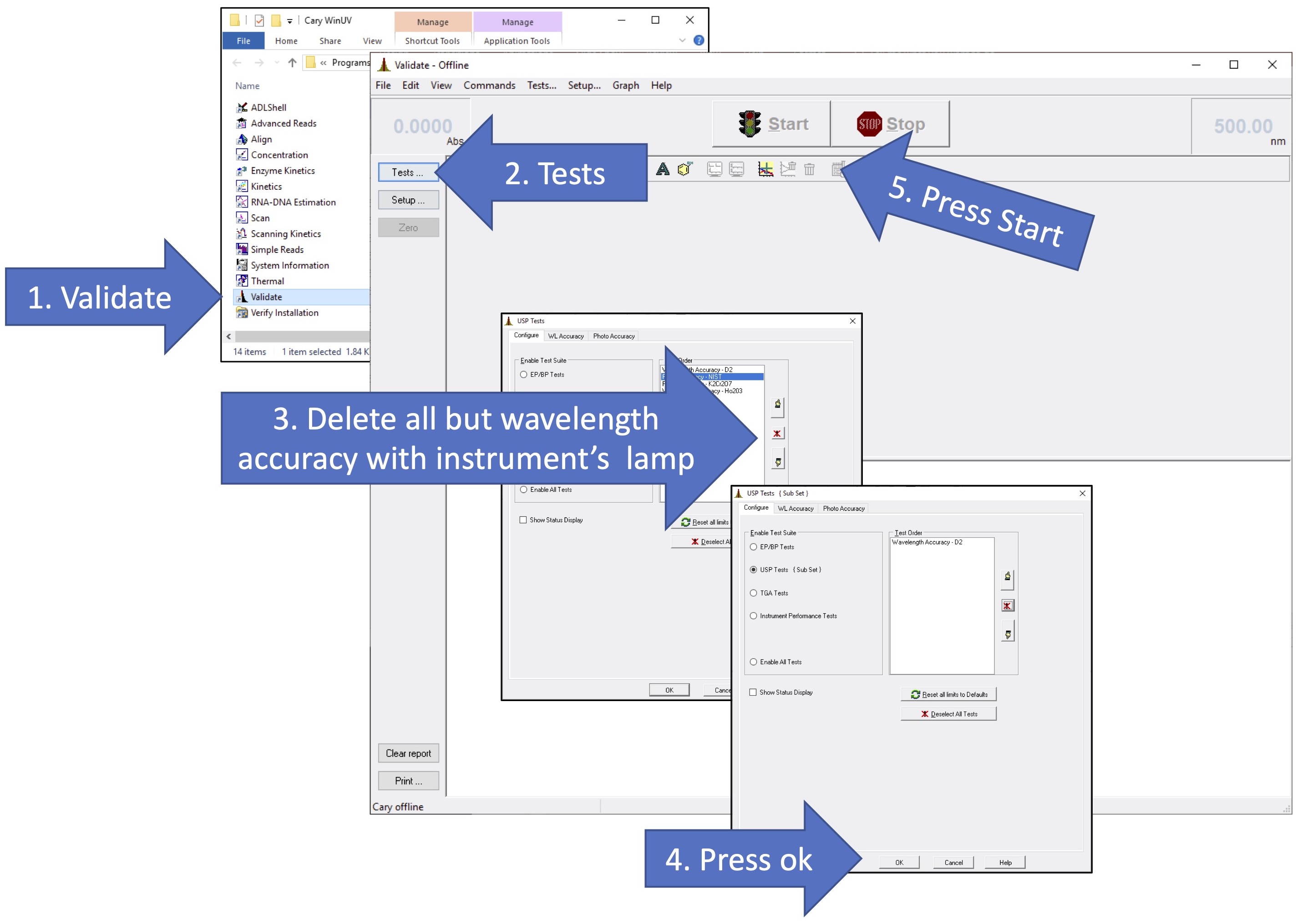
Prior to using any instrument, you should run checks to ensure the instrument is functioning properly. While the Cary UV-vis instruments run initialization procedures upon startup, there is a "Validate" program that will validate the instrument's performance. You should run a wavelength validation after the instrument has warmed up (if applicable). For Cary 100 instruments, use the deuterium (D2) lamp to validate wavelength accuracy. For the Cary 60, use the xenon (Xe) lamp to calibrate wavelength accuracy. The figure below gives a summary of the steps involved in validating the instrument.

1. Find the "Cary WinUV" shortcut on the computer desktop and open it. The linked folder contains all the programs that operate the Cary spectrophotometer. Open the "Validate" Program.
   • The Validate window should open. At the top left corner of the window, it should say "Validate-Online". If it says otherwise (ie "Validate-Offline, as pictured below) then it is not connected to the instrument. Wait a few moments to see if it connects. In the meantime, make sure the instrument is powered on. If it does not connect, try pressing "connect" (its where the start button is), and if that fails, get help.
2. On the left hand side of the Validate Window, choose "Tests".
   • The Tests window will open. Choose "Instrument Performance Tests".
   • There should be a list of several available tests in the "Test Order" box. If there is not, double check that the instrument is "online". Then, press the "Reset all limits to Default button" - this usually regenerated the list of available tests.
3. It is sufficient to run one wavelength validation test. In the "Test Order" box, choose the wavelength accuracy test that uses the instrument's own lamp (either D2 or W). To do this, you should remove all other tests by selecting each and pressing the "remove test" button that is just to the right of the box (it looks like an exclamatino point with a red "X". Do this until the test you want is the only one remaining.
4. Press "OK" after you have specified the validation test to be run.
   • The USP Tests box will close.
5. Check to make sure there are no samples in the light path. Close the sample compartment. Then Press "Start".
   • This should initiate data collection. It will take a few minutes, and during this time you should be able to see the collected spectrum recorded on the screen. If not, get help.

Figure \(\PageIndex{1}\): A visual summary of steps involved in validating the Agilent Cary UV-vis spectrophotometers. (CC-BY-NC-SA; Kathryn Haas)

After the validation, copy and paste the relevant data and images from the report into your ELN.

Collect the Absorption Spectrum of Iodine Vapor

1. Load the Scan Software by clicking the icon on the Windows main screen. In a few moments the scan software main screen will appear and will begin to communicate with the instrument. You can follow the progress by monitoring the display at the lower left of the screen. When the traffic light at the top center of the screen turns green, the system is ready. You will see absorbance at the upper left and wavelength at the upper right of the screen.

Figure \(\PageIndex{4}\): The Scan Module Main Screen. (CC-NC-BY-DUKE CHEM)

2. Click the button and wait for the setup screen to appear. Select, first, the Cary tab to begin setting parameters for your sample runs. Under Xmode, the Mode should be set to nanometers and your scan range from 620 to 490. Under Ymode, the Mode should be set to absorbance and the range from 0.02 to 0.25. The Ave time should be 0.1 seconds and the Data interval should be set to 0.1 nm. This will yield a Scan Rate of 60 nm/min.

Figure \(\PageIndex{5}\): The Scan Setup Screen. (CC-NC-BY-DUKE CHEM)

3. Select the Options tab on the setup screen and set the Spectral Band Width (SBW) to 0.2 nm. Select Double Beam Mode. Select UV-Vis as the source and be sure the Source changeover is set to 350 nm. Under Display options you can choose Individual data.

Figure \(\PageIndex{6}\): The Options Tab of the Scan Setup Screen. (CC-NC-BY-DUKE CHEM)

4. Select the Reports tab. Put your names in the Name box and the title of the experiment in the Comment box. Under Options, check Data Form, Graph, Focused trace. and % Page Height 50. Be sure the Include XY pairs table is not checked. Click Peak Information. Under Peak Table, put a check in All peaks, set the Threshold to 0.0200, and put Peaks in the Peak Type box. Click to return to the Setup screen. Choose Select for ASCII (csv). Click to return to the main screen.

Figure \(\PageIndex{7}\): The Reports Tab of the Scan Setup Screen. (CC-NC-BY-DUKE CHEM)

5. Remove the 1 cm cuvette holder from the Sample (front) beam of the instrument and replace it with the 10 cm sample cell holder. Place your iodine vapor sample in the Sample holder and close the cover. Click to begin your run. You will be prompted for a filename. After naming the file you will be prompted for a sample name. Place the name of the sample (Iodine) in this box. As the run proceeds you will see the spectrum generated in real time on the screen.

Figure \(\PageIndex{8}\): The Absorption Spectrum of Iodine Vapor. (CC-NC-BY-DUKE CHEM)

6. At the conclusion of the run, find the \(\upsilon^{\prime\prime}=0 \;\; to \;\; \upsilon^{\prime}=25\) transition that is expected to occur at 545.5 nm. Add an annotation to the spectrum to indicate this peak on your spectrum. Also locate the wavelength showing the largest absorption intensity and label it on your spectrum (see note below).

Note

Since the baseline is not straight, the peak of largest absorption intensity is found by consideration of both the base and the peak height.

7. Remove the sample and sample holder and replace the 1 cm cuvet sample holder in the instrument, using the screw to secure it properly.
8. Be sure you have screenshots of the needed results, and the Excel spreadsheet generated at the end of the run. Exit the software and turn off the instrument.

Instructions for Data Analysis (Part I Absorption Spectra of Iodine)

Note

• Do not forget to make corrections to the wavelengths based on the results of the validation experiment.

• Be careful not to confuse peaks originating from \(\upsilon^{\prime\prime}=0\) with those of "hot bands" originating from \(\upsilon^{\prime\prime}>0\).
• You may consult your instructors and classmates during data analysis, however all work should be your own.

1. Given that the \(\upsilon^{\prime\prime}=0\) to \(\upsilon^{\prime}=25\) transition occurs at 545.5 nm, assign the peaks in the spectrum according to their \(\upsilon^{\prime}\) values.
2. Choose 20 peaks:
   • Convert their wavelengths to wavenumbers. These are the values of \(G_{\upsilon}\).
   • Calculate \(\Delta G_{\left ( \upsilon \right )}\)  (see Equation 5.3.5)
3. Using MATLAB plot \(\Delta G_{\left ( \upsilon \right )}^{\prime}\) (wavenumbers) vs \(\left (\upsilon^{\prime}+1 \right )\) (see Equation 5.3.5). Perform a linear least squares regression and overlay the fitted line on the plot of the data.
4. From the intercept calculate \(\omega_{e}^{\prime}\) using Equation 5.3.5.
5. From the slope calculate \(\chi_{e}^{\prime}\) using Equation 5.3.5.
6. From Equation 5.3.7 calculate \(D_{e}^{\prime}\).
7. Estimate your error in measuring the peak positions. Using the standard deviation of the slope and intercept, and Equation 5.3.5, calculate the uncertainties in \(\omega_{e}^{\prime}\), \(\chi_{e}^{\prime}\) and \(D_{e}^{\prime}\).
8. Calculate the Morse parameter, \(a^{\prime}\) from equation Equation 5.3.7.
9. Compare your results with literature values (Ref. 8, p. 540, and Ref. 4).

 Discussion Questions

Include responses to the following in your ELN.

1. Determine the value of \(\nu_{00}\) (the energy of the transition from \(\upsilon^{\prime\prime}=0\) to \(\upsilon^{\prime}=0\)) by appropriate substitution into Equation 5.3.4.

   Note

   To do this you will need to have already done the data analysis for Part II and will also need Equation 5.3.8.

2. Why do the vibrational spacings get narrower as V(R) increases?
3. Why is the Morse potential asymmetric?
4. Why are some of the transitions called "Hot Bands"?
5. How would you calculate \(\chi_{e}^{\prime\prime}\) and \(D_{e}^{\prime\prime}\) using the hot bands?. (See reference 6 for help.)
6. What are the units of the Morse parameter, a, in Equation 5.3.7?