1.5: Polarity of bonds and molecules

Polar covalent bonds

Formal charge calculations assume the covalent bonds are equally distributed between the bonded atoms. It is true only when the two bonded atoms are the same. Different atoms have different abilities to attract the bonded electrons, which is measured in terms of electronegativity (\(\chi\)).

Electronegativity

Electronegativity is the ability of an atom to draw bonded electrons to itself.

There are different scales developed to calculate the electronegativity. Figure 1.5.1 shows electronegative values using the most common Pauling electronegativity scale.

Figure \(\PageIndex{1}\): Periodic table of electronegativity (\(\chi\)) values by Pauling scale. (Copyright; Cooper.dav.j, CC0, via Wikimedia Commons)

When the bonded atoms are the same, e.g., \(\ce{Cl-Cl}\), the electronegativity difference \(\Delta\chi\) is zero, and the bond is a pure covalent bond. When the bonded atoms are different, e.g., \(\ce{H-Cl}\) the bonded electrons are nearer the more electronegative atom, creating a dipole with a partial negative (\(\delta -\)) end on the more electronegative atom and a partial positive (\(\delta +\)) end on the more electropositive atom. The bond dipole is show by \(\delta +\) and \(\delta -\) signes on electropositive and electronegative atoms, as in \(\ce{\overset{\delta{+}}{H}{-}\overset{\delta{-}}{Cl}}\) or by a Polarity vector starting with a plus sing on the tail over the more electropositive atom and the arrow head on the more electronegative atom as in \(\ce{\overset{\Large{+\!->}}{H-Cl}}\). However, for a slight difference of \(\Delta\chi\), less than 0.5, is considered a covalent bond. A \(\Delta\chi\) between 0.5 and 1.7 is a polar covalent. For a large \(\Delta\chi\) more than 1.7, the bonding electrons are considered transferred to the more electronegative atom, resulting in an ionic bond. Figure 1.5.2 illustrates \(\ce{Cl-Cl}\) bond having \(\Delta\chi\) = 0 as covalent, \(\ce{H-Cl}\) having \(\Delta\chi = 3.16 - 2.2 =0.94\) as polar covalent, and \(\ce{NaCl}\) having \(\Delta\chi\ = 3.16 - 0.93 = 2.23\) as ionic bond.

Figure \(\PageIndex{2}\): Illustrates of a covalent \(\ce{Cl-Cl}\) bond having \(\Delta\chi\) = 0, a polar covalent \(\ce{H-Cl}\) bond having \(\Delta\chi = 3.16 - 2.2 =0.94\), and an ionic \(\ce{NaCl}\) bond having \(\Delta\chi\ = 3.16 - 0.93 = 2.23\). (Copyright; Public domain)

Caution

The \(\Delta\chi\) numbers between 0.5 and 1.7 should be considered as a rough guide, not as sharp cutoff points, because there is a diffused boundary between covalent and polar covalent, as well as between polar covalent and ionic bond. For example, \(\ce{H3C-Li}\) bond is drawing as a polar covalent \(\ce{H3\overset{\delta{-}}{C}{-}\overset{\delta{+}}{Li}}\), as well as as ionic \(\ce{H3C^{-}Li^{+}}\), and both ways are acceptable.

Molecular orbital theory explains the polarity of a bond related to the difference in the energy of the valence orbitals of the combining atoms. In the case of the nonpolar covalent bond, the bonding atomic orbitals are of similar energy, and the molecular orbital is equally lower than them in energy, as illustrated in Figure 1.5.3. In the case of a covalent bond, the valence atomic orbital of an electronegative atom is lower in energy due to a stronger attraction to the nuclei than that of the electropositive atom. The bonding molecular orbital has a lower energy than both atomic orbitals, but is closer to that of the electronegative atom. The molecular orbital has more character of the atomic orbital that is closer to it in energy. In other words, the electrons in the bonding orbitals are more on the electronegative atom than on the electropositive, resulting in the bond polarity.

Figure \(\PageIndex{3}\): Depiction of a MO diagram of a covalent bond (left), e.g., as in \(\ce{H-H}\) and a polar covalent bond (right), as in \(\ce{H-Cl}\). In both cases, a bond is a shared pair of electrons. (Copyright; Krishnavedala, Public domain, via Wikimedia Commons)

Electrostatic potential map

The polarity of the bonds and molecules can be visualized using electrostatic potential (ESP) maps, which display their electrostatic potential through color schemes. Red typically represents an electron-rich region (negative potential), green is neutral, and blue is an electron-deficient region (positive potential). Figure 1.3.4 displays electrostatic potential maps of \(\ce{H3C-I}\), \(\ce{H3C-Br}\), \(\ce{H3C-Cl}\), and \(\ce{H3C-F}\), respectively. The \(\Delta\chi\) increases in the order \(\ce{H3C-I}\) < \(\ce{H3C-Br}\) < \(\ce{H3C-Cl}\) < \(\ce{H3C-F}\), which is reflected in the ESP maps by increasing \(\delta -\) (red region) on halogen and increasing \(\delta +\) (blue region) on carbon end of the electron cloud in the same order.

Figure \(\PageIndex{4}\): Electrostatic potential maps showing increasing polarity of \(\ce{C-X}\) bond (from left to right) in the order \(\ce{H3C-I}\) < \(\ce{H3C-Br}\) < \(\ce{H3C-Cl}\) < \(\ce{H3C-F}\). The color scale is shown in the bar below each figure. (Copyright: Public domain).

Caution

Electrostatic potential maps (ESP) are comparable only if they were prepared by using the same color scale. Do not compare the ESP maps from different books or different pages or figures of the same book as the color schemes may be different.

Bond dipole moment \(\mu\)

Bond dipole moment (\(\mu\) is a measure of the polarity of a chemical bond, calculated by the following formula: \(\mu = \delta\times d\), where \(\delta\) is the charge (either \(\delta +\) or \(\delta -\) as both have the same magnitude) and \(d\) is the distance between the centers of positive and negative charge, i.e., bond length. SI unit of \(\mu\) is Coulomb-meter (C m), but the commonly used unit is Debye (D), where 1D = 3.336 x 10^-30 C m.

Dipole moment is a vector quantity. For a molecule having more than one polar bond, the vector addition of individual bond dipole moments gives the dipole moment of the molecule. However, for diatomic molecules, the dipole moment of the bond is the dipole moment of the molecule, which varies from 0D to 11D. For example, dipole moment of Nonpolar \(\ce{Cl-Cl}\) is 0D and on the other extreme the dipole moment of ionic \(\ce{Na^{+}Cl^{-}}\) is 9.001D.

The dipole moment of a molecule can be measured in the laboratory. The experimental measured dipole moment (\(\mu_{observed}\) is usually less than theoretical dipole moment (\(\mu_{theoretical}\)) calculated by assuming the \(\delta -\) is equal to charge of an electron (1e), i.e., 1.6022 x 10^-19 C and \(d\) is the bond length, assuming an electron is completely transferred in the ionic bond. It allows for calculating the percentage ionic character of the bond using the following formula.

\[\text{% Ionic character} = \frac{\mu_{observed}}{\mu_{theoretial}}\times 100\nonumber\]

Example \(\PageIndex{1}\)

a) Given the bond distance of \(\ce{H-Cl}\) is 1.275 Å and charge on an electron (1e) is 1.6022 x 10^-19 C, what will be its theoretical dipole moment \(\mu_{theoretical}\) if it was 100% ionic? b) Given the observed dipole moment \(\mu_{observed}\) is 1.03 D, what is the % ionic character and what is the % covalent character of \(\ce{H-Cl}\)

Solution

a)

Given:

\(d = 1.275\AA = \frac{1.275\AA\times 1\text{m}}{10^{10}\AA} = 1.275 \times 10^{-10}\text{m}\)

\(\delta\) = 1.6022 x 10^-19 C

Calculations: \(\mu_{theoretical} = \delta\times d = 1.275 \times 10^{-10}\text{m}\times 1.6022\times 10^{-19}\text{C} = 2.0428\times 10^{-29} \text{ C m}\)

b)

Given:

\(\mu_{observed} = \frac{1.03\text{D}\times 3.336\times 10^{-30}\text{C m}}{1\text{D}} = 3.436 \times 10^{-30}\text{ C m}\)

Calculations: \(\text{% Ionic character} = \frac{\mu_{observed}}{\mu_{theoretial}}\times 100 = \frac{3.436\times 10^{-30}\text{C m}}{2.0428 \times 10^{-29} \text{ C m}}\times 100 = 17\%\)

\(\text{% covalent character = 100 - % Ionic character} = 100 - 17 = 83\%\)

Example \(\PageIndex{2}\)

a) Given the bond distance of \(\ce{Na^{+}Cl^{-}}\) is 2.361 Å and charge on an electron (1e) is 1.6022 x 10^-19 C, what will be its theoretical dipole moment \(\mu_{theoretical}\) if it was 100% ionic? b) Given the observed dipole moment \(\mu_{observed}\) is 9.001 D, what is the % ionic character and what is the % covalent character of \(\ce{H-Cl}\)

Solution

a)

Given:

\(d = 2.361\AA = \frac{2.361\AA\times 1\text{m}}{10^{10}\AA} = 2.361 \times 10^{-10}\text{m}\)

\(\delta\) = 1.6022 x 10^-19 C

Calculations: \(\mu_{theoretical} = \delta\times d = 2.361 \times 10^{-10}\text{m}\times 1.6022\times 10^{-19}\text{C} = 3.783 \times 10^{-29} \text{ C m}\)

b)

Given:

\(\mu_{observed} = \frac{9.001\text{D}\times 3.336\times 10^{-30}\text{C m}}{1\text{D}} = 3.003 \times 10^{-29}\text{ C m}\)

Calculations: \(\text{% Ionic character} = \frac{\mu_{observed}}{\mu_{theoretial}}\times 100 = \frac{3.003\times 10^{-29}\text{C m}}{3.783 \times 10^{-29} \text{ C m}}\times 100 = 79\%\)

\(\text{% covalent character = 100 - % Ionic character} = 100 - 78 = 21\%\)

The above two examples clarify that polar covalent bonds have some ionic character and ionic bonds have some covalent character. For example, covalent \(\ce{\overset{\delta{+}}{H}{-}\overset{\delta{-}}{Cl}}\) has 17% ionic character, and ionic \(\ce{Na^{+}Cl^{-}}\) has 20% covalent character.

Polar molecules

Polarity is a vector quantity. If there is more than one polar bond in a molecule, the polarity of the molecule is a result of the vector addition of the individual bond polarities. Therefore, the polarity of a molecule is determined by the following general rules.

• A molecule having no polar bonds is nonpolar.
• A molecule having one polar bond is polar.
• A non-symmetric molecule having more than one polar bond is usually polar because the individual bond polarities typically do not entirely cancel each other, but,
  • A symmetric molecule having more than one polar bond is non-polar because the individual bond polarities cancel each other.

Examples of nonpolar molecules having no polar bonds are \(\ce{Cl-Cl}\), \(\ce{CH4}\), etc. Examples of polar molecules having one polar bond include \(\ce{\overset{\Large{+\!->}}{H-Cl}}\), \(\ce{H3\overset{\Large{+\!->}}{C-Cl}}\), etc.

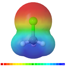
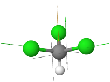
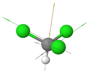
Examples of polar non-symmetric molecules having more than one polar bond include \(\ce{CCl3H}\) with tetrahedral geometry but one \(\ce{C-H}\) bond different than the others, \(\ce{NH3}\) with trigonal pyramidal geometry and the fourth electron domain is a lone pair, \(\ce{H2O}\) with bent geometry having to bonding pairs and two lone pairs in a tetrahedral electron group geometry, etc., as illustrated in the Figure 1.5.5.

\(\ce{CCl3H}\)

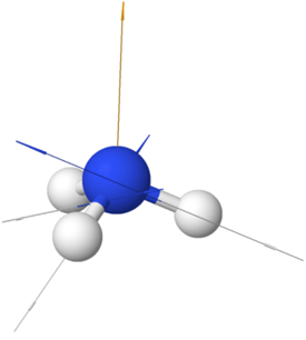\(\ce{:\!NH3}\)

\(\ce{H2\overset {\cdot\cdot}{O}:}\)

Figure \(\PageIndex{5}\): Examples of polar non-symmeric molecuels haivng more than one polar bonds: \(\ce{CCl3H}\) with one bond different than the other three, \(\ce{:\!NH3}\) with one lone pair and three polar bonds, and \(\ce{H2\overset {\cdot\cdot}{O}:}\) with two lone pairs and two polar bonds. The individual bond polarities are shown by the arrows of the same color as the atoms in the models, and the orange arrow indicates the overall polarity, drawn using the online app https://molview.org (Copyright: Public domain).

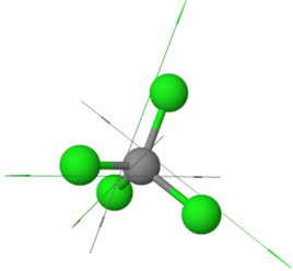
Examples of symmetric nonpolar molecules having all equal polar bonds include those having two equal bonds in a linear geometry, e.g., \(\ce{O=C=O}\), three equal bonds in a triangular planar geometry, e.g., \(\ce{BF3}\), four equal bonds in a tetrahedral geometry, e.g., \(\ce{CCl4}\), etc., as illustrated in Figure 1.5.6.

\(\ce{O=C=O}\)

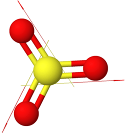\(\ce{O=\overset{\!\!\overset{\huge {\:O}}|\!\!|\,}{S}=O}\)

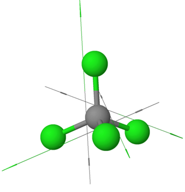\(\ce{CCl4}\)

Figure \(\PageIndex{6}\): Examples of symmetric nonpolar molecules having all equal polar bonds. Arrows show individual bond polarity vectors drawn using the online app https://molview.org (Copyright: Public domain).

The set of molecular polarities compared in Figure 1.5.7 demonstrates the partial or full cancellation of individual bond polarities within a molecule. \(\ce{CH3Cl}\) has one polar \(\ce{C-Cl}\) bond and dipole moment \(\mu\) = 1.20D, while \(\ce{CH2Cl2}\) has two polar \(\ce{C-Cl}\) bonds, but the dipole moment is not twice because the two bond polarity vectors partially cancel each other. \(\ce{CHCl}\) has three polar \(\ce{C-Cl}\) bonds, but the \(\mu\) = 1.20D equal to one polar \(\ce{C-Cl}\) bond, and \(\ce{CCl4}\) has four polar \(\ce{C-Cl}\) bonds, but is a nonpolar molecule because the individual bond dipole vectors cancel each other in this symmetric molecule.

\(\ce{CH3Cl}\), dipole moment \(\mu\) = 1.20D

\(\ce{CH2Cl2}\), dipole moment \(\mu\) = 1.68D

\(\ce{CHCl3}\), dipole moment \(\mu\) = 1.20D

\(\ce{CCl4}\), dipole moment \(\mu\) = 0.01D

Figure \(\PageIndex{7}\): Illustration of bond polarities indicated by arrows of the same color as the bonded atom and the overall bond polarity by orange arrows, and dipole moments for \(\ce{CHCl3}\), \(\ce{CH2Cl2}\), \(\ce{CHCl3}\), and \(\ce{CCl4}\) Arrows showing polarity vectors were drawn using the online app https://molview.org, and the dipole moments \(mu\) were calculated using online app https://molcalc.org/ (Copyright: Public domain).

Intermolecular forces

Intermolecular forces are the electrostatic interactions between molecules. The intermolecular forces are usually much weaker than the chemical bonds (intramolecular forces), but still, they play an important role in determining the properties of the compounds. The major intermolecular forces include London dispersion forces, dipole-dipole interactions, and hydrogen bonding.

London dispersion forces

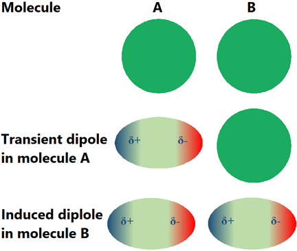
The electron cloud around atoms is not always symmetrical around the nuclei. It temporarily sways to one side or the other, generating a transient dipole. The transient dipole induces a dipole in the neighboring molecule, resulting in an attractive force between the opposite poles, called the transient dipole-induced dipole interaction, London dispersion force, or van der Waals’ force, as illustrated in Fig. 1.5.8. Although London dispersion forces are transient, they keep reappearing randomly.

London dispersion forces are not unique to nonpolar molecules; they are present in all types of molecules, but these are the only intramolecular forces present in nonpolar molecules.

Figure \(\PageIndex{8}\): Illustration of transient dipole-induced dipole, i.e., London dispersion forces (Copyright: Public domain).

Effect of London dispersion forces on melting point (MP) and boiling point (BP)

London dispersion forces are responsible for maintaining the molecules in a solid or liquid state at lower temperatures. At higher temperatures, thermal forces become stronger and separate the molecules to larger distances, with almost no intermolecular interactions in the gas state. Therefore, melting point and boiling point values are indicators of the intermolecular forces in the compounds.

Since molecular weight (MW) is directly proportional to the number of electrons, London dispersion forces and, consequently, the melting point and boiling points are directly proportional to molecular weight, i.e., the higher the molecular weight, the higher the melting and boiling point.

Figure 1.5.9 shows that the molecular weight gradually increases from compounds I to IV, V, and VI; the melting points and the boiling points also increase in the same order.

Figure \(\PageIndex{9}\): Illustration of i) increase in melting and boiling points of example organic compounds with increase in their molecular weights (compare compounds I, II, IV, V, and VI) and ii) decrease in melting and boiling points with increase in branching for the same molecular weight (compare compounds II, III, and IV (Copyright; Public domain).

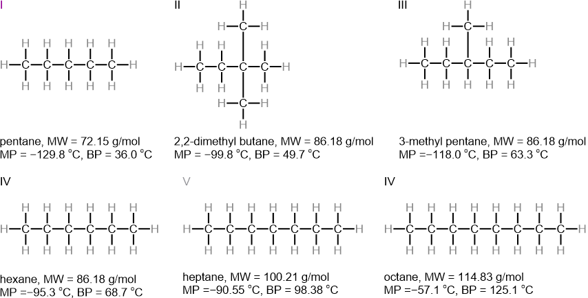
The transient dipole induces a dipole in the neighboring molecule through surface-to-surface contact. Therefore, linear chain organic molecules having a cylindrical shape with a larger surface area have higher melting and boiling points than branched molecules of the same molecular weight having a globular shape that can make less area of contact with the neighboring molecules.

For example, melting and boiling points decrease as the branching increases from IV to III to II in Figure 1.5.9.

Note that the effect of molecular weight is stronger than the effect of branching on the melting and boiling points.

For example, the melting points of compounds II, III, and IV, having the same molecular weights, are higher than that of compound I, which has a lower molecular weight, and lower than that of compound V, which has a higher molecular weight.

Dipole-dipole interactions

Polar molecules have permanent dipoles; one end of the molecule is partially positive (δ+) and the other is partially negative (δ-). The polar molecules have dipole-dipole interaction, i.e., electrostatic attraction between opposite partial charges on the dipoles, in addition to transient dipole-induced dipole interactions, as illustrated by dotted line in the figure on the right. The polar molecules orient in a way to maximize the attractive forces between the opposite charges and minimize the repulsive forces between the same charges, as illustrated in the figure on the left (Copyright: Public domain).

Polar molecules usually have higher melting and boiling points than nonpolar molecules of comparable molar mass. For example, a nonpolar butane has significantly lower melting and boiling points (mp = -137 ^oC, bp = 0 ^oC) compared to polar acetone (mp = -94.9 ^oC, bp = 56.1 ^oC) of the same molar mass, but having a polar \(\ce{\overset{\delta +}{C}=\overset{\delta -}{O}}\) group, as illustrated in the figure on the right (Copyright: Public domain). Note, in the electrostatic potential maps shown in the figure on the right, green is neutral, blue is \(\delta +\), and red is \(\delta -\).

Hydrogen bonds

Hydrogen bonding is a dipole-dipole interaction between \(\ce{\overset{\delta+}{H}}\) of \(\ce{\overset{\delta -}{X}-\overset{\delta +}{H}}\) bond with the \(\ce{\overset{\delta-}{X}}\) of a neighboring molecule, where \(\ce{X}\) is \(\ce{N}\), \(\ce{O}\), or \(\ce{F}\), as illustrated by dotted lines between \(\ce{H2O}\) molecules in he figure on the right (Copyright: Magasjukur2 / Public domain, via Wikimedia Commons). Although a hydrogen bond is a dipole-dipole interaction, it is distinguished from the usual dipole-dipole interactions because of the following special features.

1. The electronegativity difference between \(\ce{H}\) and \(\ce{N}\), \(\ce{O}\), or \(\ce{F}\) is typically greater than that of other polar bonds.
2. The charge density on \(\ce{\overset{\delta+}{H}}\) is higher due to the smaller size than on other dipoles.
3. Because of its smaller size, \(\ce{-\overset{\delta+}{H}}\) can penetrate less accessible spaces to interact with the \(\ce{\overset{\delta-}{N}}\), \(\ce{\overset{\delta-}{O}}\), or \(\ce{\overset{\delta-}{F}}\) of the other molecule.

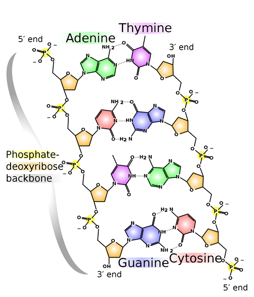
A hydrogen bond is usually stronger than the usual dipole-dipole interactions. For example, it is reflected by higher melting and boiling points of hydrogen-bonded ethanol (mp = -114.1 ^oC, bp = 78.2 ^oC) higher than polar ethanal (mp = -123.4 ^oC, bp = 20.2 ^oC), and nonpolar propane (mp = -187.7 ^oC, bp = -42.0 ^oC) of comparable molar masses. Hydrogen bonding is the most common and essential intermolecular interaction in biomolecules. For example, two strands of DNA molecules are held together through hydrogen bonding, as illustrated in Figure 1.5.10. Proteins also acquire structural features needed for their functions mainly through hydrogen bonding.

Figure \(\PageIndex{10}\): Chemical structure of DNA, with a colored label identifying the four bases as well as the phosphate and deoxyribose components of the backbone. Dotted lines are the hydrogen bonds holding the two strands of DNA together. Source: Madprime (talk · contribs) / CC0

Effect of multiple factors on intermolecular forces

The effect of multiple factors on intermolecular forces usually adds up. For example, nonpolar hexane has a lower melting point and boiling point than polar pentanal, which, intrinsically, has a lower melting point than hydrogen-bonded pentan-1-ol of comparable molar masses, as listed in Table 1.5.11. Butanoic acid acid of similar molar mass has significantly higher melting and boiling point than pentan-1-ol, bucause it has a polar \(\ce{\overset{\delta{+}}{C}{=}\overset{\delta{-}}{O}}\), and a hydrogen bonding \(\ce{-\overset{\delta{-}}{O}{-}\overset{\delta{+}}{H}}\) in one molecule, i.e., in \(\ce{-\!\!{\overset{\overset{\huge\enspace\!{\overset{\Large{\delta{-}}}{O}}}|\!\!|\enspace}{\overset{\delta{+}}{C}}}\!\!-\overset{\delta{-}}{O}-\overset{\delta{+}}{H}}\) group. Similarly, butan-1,4-diol having two hydrogen bonding \(\ce{-\overset{\delta{-}}{O}{-}\overset{\delta{+}}{H}}\) groups in one molecule, has higher melting and boiling points than butanoic acid, as listed in Table \(\PageIndex{11}\)

Table \(\PageIndex{11}\): Compares boiling points and solubility of a carboxylic acid, alcohol, and aldehyde of comparable molar mass.

Condensed formula	IUPAC name	Molar mass (g/mol)	Melting point (^oC)	Boiling point (^oC)	Solubility in water
\(\ce{HO(CH2)4OH}\)	Butan-1,4-diol	90.1	20.1	235	Miscible
\(\ce{CH3(CH2)2COOH}\)	Butanoic acid	88.1	-5.1	164	Miscible
\(\ce{CH3(CH2)3CH2OH}\)	Pentan-1-ol	88.2	-78	138	22 g/L
\(\ce{CH3(CH2)3CHO}\)	Pentanal	86.1	-60	103	14 g/L
\(\ce{CH3(CH2)4CH3}\)	Hexane	86.2	-95	69	Immiscible

Effect of intermolecular forces on solubility

A general rule of thumb, "like dissolves like," means polar compounds are soluble in polar solvents and nonpolar compounds in nonpolar solvents. For example, nonpolar hexane is soluble in nonpolar toluene but immiscible in polar water. Pentanal having a polar \(\ce{-\!\!{\overset{\overset{\huge\enspace\!{\overset{\Large{\delta{-}}}{O}}}|\!\!|\enspace}{\overset{\delta{+}}{C}}}\!\!-{H}}\) group and butanol having hydrogen bonding \(\ce{\overset{\delta{-}}{O}{-}\overset{\delta{+}}{H}}\) group are partially soluble in polar water, as listed in Table \(\PageIndex{11}\). Butanoic acid having a polar \(\ce{\overset{\delta{+}}{C}{=}\overset{\delta{-}}{O}}\), and a hydrogen bonding \(\ce{-\overset{\delta{-}}{O}{-}\overset{\delta{+}}{H}}\) group and butan-1,4-diol having two hydrogen bonding \(\ce{-\overset{\delta{-}}{O}{-}\overset{\delta{+}}{H}}\) groups are missible in water, as listed in Table \(\PageIndex{11}\). Note that all the compounds listed in Table \(\PageIndex{11}\) have similar molar masses.

Polar organic compounds usually have a polar head that tends to dissolve in polar solvents like water but not in nonpolar solvents like toluene, and a nonpolar tail that tends not to dissolve in polar solvents but dissolves in nonpolar solvents. \[\ce{\underbrace{CH3CH2CH2CH2}_{Nononpolar\: tail}-\!\!\underbrace{\overset{\delta{-}}{O}{-}\overset{\delta{+}}{H}}_{Polar\: head}}\nonumber\] The factors contradict, and the overall solubility is determined by which one is stronger. When the nonpolar tail is small, up to three or four carbons, the effect of the polar head is strong, making the compound soluble in water. When the nonpolar tail is medium size, from ~4 to ~7, the compounds are partially soluble in water. When the nonpolar tail is large, the compounds are immiscible in water, as illustrated in Table \(\PageIndex{12}\).

Table \(\PageIndex{12}\): Melting points, boiling points, and solubility of alcohols in water (Note: Miscible means make a solution in all proportions, and immiscible have solubility less than 1 g/L)

Formula	Boiling point (^oC)	Melting point (^oC)	Solubility in water (g/L) at 25 ^oC
\(\ce{CH3OH}\)	64.8	-97	Miscible
\(\ce{C2H5OH}\)	78.5	-114	Miscible
\(\ce{C3H7OH}\)	97	-126	Miscible
\(\ce{C4H9OH}\)	117	085	73
\(\ce{C5H11OH}\)	138	-79	22
\(\ce{C6H13OH}\)	157	-48	5.9
\(\ce{C7H15OH}\)	175	-35	1.7
\(\ce{C8H17OH}\)	195	-16	immiscible
\(\ce{C9H19OH}\)	212	-5.1	immiscible
\(\ce{C10H212OH}\)	232	6.4	immiscible