
14.3: Laminar and Turbulent Flow
- Page ID
- 294336

\( \newcommand{\vecs}[1]{\overset { \scriptstyle \rightharpoonup} {\mathbf{#1}} } \)
\( \newcommand{\vecd}[1]{\overset{-\!-\!\rightharpoonup}{\vphantom{a}\smash {#1}}} \)
\( \newcommand{\id}{\mathrm{id}}\) \( \newcommand{\Span}{\mathrm{span}}\)
( \newcommand{\kernel}{\mathrm{null}\,}\) \( \newcommand{\range}{\mathrm{range}\,}\)
\( \newcommand{\RealPart}{\mathrm{Re}}\) \( \newcommand{\ImaginaryPart}{\mathrm{Im}}\)
\( \newcommand{\Argument}{\mathrm{Arg}}\) \( \newcommand{\norm}[1]{\| #1 \|}\)
\( \newcommand{\inner}[2]{\langle #1, #2 \rangle}\)
\( \newcommand{\Span}{\mathrm{span}}\)
\( \newcommand{\id}{\mathrm{id}}\)
\( \newcommand{\Span}{\mathrm{span}}\)
\( \newcommand{\kernel}{\mathrm{null}\,}\)
\( \newcommand{\range}{\mathrm{range}\,}\)
\( \newcommand{\RealPart}{\mathrm{Re}}\)
\( \newcommand{\ImaginaryPart}{\mathrm{Im}}\)
\( \newcommand{\Argument}{\mathrm{Arg}}\)
\( \newcommand{\norm}[1]{\| #1 \|}\)
\( \newcommand{\inner}[2]{\langle #1, #2 \rangle}\)
\( \newcommand{\Span}{\mathrm{span}}\) \( \newcommand{\AA}{\unicode[.8,0]{x212B}}\)
\( \newcommand{\vectorA}[1]{\vec{#1}} % arrow\)
\( \newcommand{\vectorAt}[1]{\vec{\text{#1}}} % arrow\)
\( \newcommand{\vectorB}[1]{\overset { \scriptstyle \rightharpoonup} {\mathbf{#1}} } \)
\( \newcommand{\vectorC}[1]{\textbf{#1}} \)
\( \newcommand{\vectorD}[1]{\overrightarrow{#1}} \)
\( \newcommand{\vectorDt}[1]{\overrightarrow{\text{#1}}} \)
\( \newcommand{\vectE}[1]{\overset{-\!-\!\rightharpoonup}{\vphantom{a}\smash{\mathbf {#1}}}} \)
\( \newcommand{\vecs}[1]{\overset { \scriptstyle \rightharpoonup} {\mathbf{#1}} } \)
\( \newcommand{\vecd}[1]{\overset{-\!-\!\rightharpoonup}{\vphantom{a}\smash {#1}}} \)
\(\newcommand{\avec}{\mathbf a}\) \(\newcommand{\bvec}{\mathbf b}\) \(\newcommand{\cvec}{\mathbf c}\) \(\newcommand{\dvec}{\mathbf d}\) \(\newcommand{\dtil}{\widetilde{\mathbf d}}\) \(\newcommand{\evec}{\mathbf e}\) \(\newcommand{\fvec}{\mathbf f}\) \(\newcommand{\nvec}{\mathbf n}\) \(\newcommand{\pvec}{\mathbf p}\) \(\newcommand{\qvec}{\mathbf q}\) \(\newcommand{\svec}{\mathbf s}\) \(\newcommand{\tvec}{\mathbf t}\) \(\newcommand{\uvec}{\mathbf u}\) \(\newcommand{\vvec}{\mathbf v}\) \(\newcommand{\wvec}{\mathbf w}\) \(\newcommand{\xvec}{\mathbf x}\) \(\newcommand{\yvec}{\mathbf y}\) \(\newcommand{\zvec}{\mathbf z}\) \(\newcommand{\rvec}{\mathbf r}\) \(\newcommand{\mvec}{\mathbf m}\) \(\newcommand{\zerovec}{\mathbf 0}\) \(\newcommand{\onevec}{\mathbf 1}\) \(\newcommand{\real}{\mathbb R}\) \(\newcommand{\twovec}[2]{\left[\begin{array}{r}#1 \\ #2 \end{array}\right]}\) \(\newcommand{\ctwovec}[2]{\left[\begin{array}{c}#1 \\ #2 \end{array}\right]}\) \(\newcommand{\threevec}[3]{\left[\begin{array}{r}#1 \\ #2 \\ #3 \end{array}\right]}\) \(\newcommand{\cthreevec}[3]{\left[\begin{array}{c}#1 \\ #2 \\ #3 \end{array}\right]}\) \(\newcommand{\fourvec}[4]{\left[\begin{array}{r}#1 \\ #2 \\ #3 \\ #4 \end{array}\right]}\) \(\newcommand{\cfourvec}[4]{\left[\begin{array}{c}#1 \\ #2 \\ #3 \\ #4 \end{array}\right]}\) \(\newcommand{\fivevec}[5]{\left[\begin{array}{r}#1 \\ #2 \\ #3 \\ #4 \\ #5 \\ \end{array}\right]}\) \(\newcommand{\cfivevec}[5]{\left[\begin{array}{c}#1 \\ #2 \\ #3 \\ #4 \\ #5 \\ \end{array}\right]}\) \(\newcommand{\mattwo}[4]{\left[\begin{array}{rr}#1 \amp #2 \\ #3 \amp #4 \\ \end{array}\right]}\) \(\newcommand{\laspan}[1]{\text{Span}\{#1\}}\) \(\newcommand{\bcal}{\cal B}\) \(\newcommand{\ccal}{\cal C}\) \(\newcommand{\scal}{\cal S}\) \(\newcommand{\wcal}{\cal W}\) \(\newcommand{\ecal}{\cal E}\) \(\newcommand{\coords}[2]{\left\{#1\right\}_{#2}}\) \(\newcommand{\gray}[1]{\color{gray}{#1}}\) \(\newcommand{\lgray}[1]{\color{lightgray}{#1}}\) \(\newcommand{\rank}{\operatorname{rank}}\) \(\newcommand{\row}{\text{Row}}\) \(\newcommand{\col}{\text{Col}}\) \(\renewcommand{\row}{\text{Row}}\) \(\newcommand{\nul}{\text{Nul}}\) \(\newcommand{\var}{\text{Var}}\) \(\newcommand{\corr}{\text{corr}}\) \(\newcommand{\len}[1]{\left|#1\right|}\) \(\newcommand{\bbar}{\overline{\bvec}}\) \(\newcommand{\bhat}{\widehat{\bvec}}\) \(\newcommand{\bperp}{\bvec^\perp}\) \(\newcommand{\xhat}{\widehat{\xvec}}\) \(\newcommand{\vhat}{\widehat{\vvec}}\) \(\newcommand{\uhat}{\widehat{\uvec}}\) \(\newcommand{\what}{\widehat{\wvec}}\) \(\newcommand{\Sighat}{\widehat{\Sigma}}\) \(\newcommand{\lt}{<}\) \(\newcommand{\gt}{>}\) \(\newcommand{\amp}{&}\) \(\definecolor{fillinmathshade}{gray}{0.9}\)- Laminar flow: Fluid travels in smooth parallel lines without lateral mixing.
- Turbulent flow: Flow velocity field is unstable, with vortices that dissipate kinetic energy of fluid more rapidly than laminar regime.
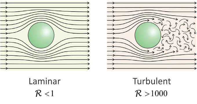
Reynolds Number
The Reynolds number is a dimensionless number is used to indicate whether flow conditions are in the laminar or turbulent regimes. It indicates whether the motion of a particle in a fluid is dominated by inertial or viscous forces.1
\[ \mathcal{R} = \dfrac{inertial\: forces}{viscous \: forces} \nonumber\]
When \(\mathcal{R}>1\), the particle moves freely, experiencing only weak resistance to its motion by the fluid. If \(\mathcal{R}<1\), it is dominated by the resistance and internal forces of the fluid. For the latter case, we can consider the limit m → 0 in eq. Error! Reference source not found., and find that the velocity of the particle is proportional to the random fluctuations: \(v(t)=f_r(t)/\zeta\).
We can also express the Reynolds number in other forms:
- In terms of the fluid velocity flow properties: \(\mathcal{R} = \dfrac{v\rho (d \overline{v}/dz)}{\eta (d^2\overline{v}/dz^2)}\)
- In terms of the Langevin variables: \(\mathcal{R} = f_{in}/f_d\).
Hydrodynamically, for a sphere of radius r moving through a fluid with dynamic viscosity η and density ρ at velocity v,
\[ \mathcal{R} =\dfrac{rv\rho}{\eta} \nonumber \]
Consider for an object with radius 1 cm moving at 10 cm/s through water: \(\mathcal{R}=10^3\). Now compare to a protein with radius 1 nm moving at 10 m/s: \(\mathcal{R}=10^{-2}\).
Drag Force in Hydrodynamics
The drag force on an object is determined by the force required to displace the fluid against the direction of flow. A sphere, rod, or cube with the same mass and surface area will respond differently to flow. Empirically, the drag force on an object can be expressed as
\[ f_d = \left[ \dfrac{1}{2} \rho C_d v^2 \right] a \nonumber \]
This expression takes the form of a pressure (term in brackets) exerted on the cross-sectional area of the object along the direction of flow, a. Cd is the drag coefficient, a dimensionless proportionality constant that depends on the shape of the object. In the case of a sphere of radius r: a = πr2 in the turbulent flow regime (\(\mathcal{R} >1000\)) Cd = 0.44–0.47. Determination of Cd is somewhat empirical since it depends on \(\mathcal{R}\) and the type of flow around the sphere.
The drag coefficient for a sphere in the viscous/laminar/Stokes flow regimes (\(\mathcal{R}<1\)) is \(C_d=24/\mathcal{R}\). This comes from using the Stokes Law for the drag force on a sphere \(f_d=6\pi \eta v r\) and the Reynolds number \(\mathcal{R}=\rho vd/\eta\).

| Reprinted with permission from Bernard de Go Mars, Drag coefficient of a sphere as a function of Reynolds number, CC BY-SA 3.0. |
________________________________
- E. M. Purcell, Life at low Reynolds number, Am. J. Phys. 45, 3–11 (1977).