
15.E: Quality Assurance (Exercises)
- Page ID
- 5345

1. Make a list of good laboratory practices for the lab accompanying this course, or another lab if this course does not have an associated laboratory. Explain the rationale for each item on your list.
2. Write directives outlining good measurement practices for a buret, a pH meter, and a spectrophotometer.
3. A atomic absorption method for the analysis of lead in an industrial wastewater has a method detection limit of 10 ppb. The relationship between the absorbance and the concentration of lead, as determined from a calibration curve, is
\[A = \mathrm{0.349 × (ppm\: Pb)}\]
Analysis of a sample in duplicate gives absorbance values of 0.554 and 0.516. Is the precision between these two duplicates acceptable based on the limits in Table 15.1?
4. The following data were obtained for the duplicate analysis of a 5.00 ppm NO3– standard.
|
sample |
X1 (ppm) |
X2 (ppm) |
|---|---|---|
|
1 |
5.02 |
4.90 |
|
2 |
5.10 |
5.18 |
|
3 |
5.07 |
4.95 |
| 4 | 4.96 | 5.01 |
| 5 | 4.88 | 4.98 |
| 6 | 5.04 | 4.97 |
Calculate the standard deviation for these duplicate samples. If the maximum limit for the relative standard deviation is 1.5%, are these results acceptable?
5. Gonzalez and colleagues developed a voltammetric method for the determination of tert-butylhydroxyanisole (BHA) in chewing gum.6 Analysis of a commercial chewing gum gave results of 0.20 mg/g. To evaluate the accuracy of their results, they performed five spike recoveries, adding an amount of BHA equivalent to 0.135 mg/g to each sample. The experimentally determined concentrations of BHA in these samples were reported as 0.342, 0.340, 0.340, 0.324, and 0.322 mg/g. Determine the percent recovery for each sample and the average percent recovery.
6. A sample is analyzed following the protocol shown in Figure 15.2, using a method with a detection limit of 0.05 ppm. The relationship between the analytical signal, Smeas, and the concentration of the analyte, CA, as determined from a calibration curve, is
\[S_\ce{meas} = \mathrm{0.273 × (ppm\: analyte)}\]
Answer the following questions if the limit for a successful spike recovery is ±10%.
(a) A field blank is spiked with the analyte to a concentration of 2.00 ppm and returned to the lab. Analysis of the spiked field blank gives a signal of 0.573. Is the spike recovery for the field blank acceptable?
(b) The analysis of a spiked field blank is unacceptable. To determine the source of the problem, a spiked method blank is prepared by spiking distilled water with the analyte to a concentration of 2.00 ppm. Analysis of the spiked method blank gives a signal of 0.464. Is the source of the problem in the laboratory or in the field?
(c) The analysis for a spiked field sample, BSF, is unacceptable. To determine the source of the problem, the sample was spiked in the laboratory by adding sufficient analyte to increase the concentration by 2.00 ppm. Analysis of the sample before and after the spike gives signals of 0.456 for B and 1.03 for BSL. Considering this data, what is the most likely source of the systematic error?
7. The following data were obtained for the repetitive analysis of a stable standard.7
|
sample |
Xi (ppm) |
sample |
Xi (ppm) |
sample |
Xi (ppm) |
|---|---|---|---|---|---|
|
1 |
35.1 |
10 |
35.0 |
18 |
36.4 |
|
2 |
33.2 |
11 |
31.4 |
19 |
32.1 |
|
3 |
33.7 |
12 |
35.6 |
20 |
38.2 |
|
4 |
35.9 |
13 |
30.2 |
21 |
33.1 |
|
5 |
34.5 |
14 |
31.1 |
22 |
36.2 |
|
6 |
34.5 |
15 |
31.1 |
23 |
36.2 |
|
7 |
34.4 |
16 |
34.8 |
24 |
34.0 |
|
8 |
34.3 |
17 |
34.3 |
25 |
33.8 |
|
9 |
31.8 |
Construct a property control chart for these data and evaluate the state of statistical control.
8. The following data were obtained for the repetitive spike recoveries of field samples.8
|
sample |
% recovery |
sample |
% recovery |
sample |
% recovery |
|---|---|---|---|---|---|
|
1 |
94.6 |
10 |
104.6 |
18 |
104.6 |
|
2 |
93.1 |
11 |
123.8 |
19 |
91.5 |
|
3 |
100.0 |
12 |
93.8 |
20 |
83.1 |
|
4 |
122.3 |
13 |
80.0 |
21 |
100.8 |
|
5 |
120.8 |
14 |
99.2 |
22 |
123.1 |
|
6 |
93.1 |
15 |
101.5 |
23 |
96.2 |
|
7 |
117.7 |
16 |
74.6 |
24 |
96.9 |
|
8 |
96.2 |
17 |
108.5 |
25 |
102.3 |
|
9 |
73.8 |
Construct a property control chart for these data and evaluate the state of statistical control.
9. The following data were obtained for the duplicate analysis of a stable standard.9
| sample | X1 (ppm) | X2 (ppm) | sample | X1 (ppm) | X2 (ppm) |
|---|---|---|---|---|---|
| 1 | 50 | 46 | 14 | 36 | 36 |
| 2 | 37 | 36 | 15 | 47 | 45 |
|
3 |
22 |
19 |
16 |
16 |
20 |
|
4 |
17 |
20 |
17 |
18 |
21 |
|
5 |
32 |
34 |
18 |
26 |
22 |
|
6 |
46 |
46 |
19 |
35 |
36 |
|
7 |
26 |
28 |
20 |
26 |
25 |
|
8 |
26 |
30 |
21 |
49 |
51 |
|
9 |
61 |
58 |
22 |
33 |
32 |
|
10 |
44 |
45 |
23 |
40 |
38 |
|
11 |
40 |
44 |
24 |
16 |
13 |
|
12 |
36 |
35 |
25 |
39 |
42 |
|
13 |
29 |
31 |
Construct a precision control chart for these data and evaluate the state of statistical control.
15.5.3 Solutions to Practice Exercises
Practice Exercise 15.1
To estimate the standard deviation we first calculate the difference, d, and the squared difference, d 2, for each duplicate. The results of these calculations are summarized in the following table.
| duplicate | d = X1 – X2 | d 2 |
|---|---|---|
|
1 |
–0.6 |
0.36 |
|
2 |
–2.3 |
5.29 |
|
3 |
0.4 |
0.16 |
|
4 |
–0.8 |
0.64 |
|
5 |
2.3 |
5.29 |
Finally, we calculate the standard deviation.
\[s=\sqrt{\dfrac{0.36+5.29+0.16+0.64+5.29}{2\times 5}}=1.08\]
Click here to return to the chapter.
Practice Exercise 15.2
Adding a 10.0-μL spike to a 10.0-mL sample is a 1000-fold dilution; thus, the concentration of added glucose is 25.0 mg/100 mL and the spike recovery is
\[\%R=\dfrac{110.3-86.7}{25.0}\times 100=\dfrac{23.6}{25.0}\times 100=94.4\%\]
Click here to return to the chapter.
Practice Exercise 15.3
The UCL is 256.9, the UWL is 254.4, the CL is 249.4, the LWL is 244.4, and the LCL is 241.9 mg glucose/100 mL. Figure 15.7 shows the resulting property control plot.
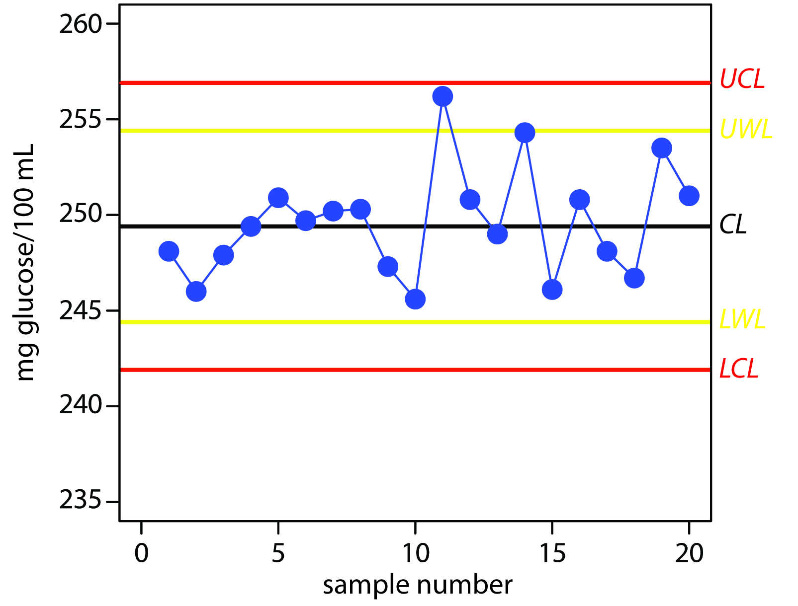
Figure 15.7 Property control plot for Practice Exercise 15.3.
Click here to return to the chapter.
Practice Exercise 15.4
Although the variation in the results appears to be greater for the second 10 samples, the results do not violate any of the six rules. There is no evidence in Figure 15.7 that the analysis is out of statistical control. The next three results, in which two of the three results are between the UWL and the UCL, violates the second rule. Because the analysis is no longer under statistical control, we must stop using the glucometer until we determine the source of the problem.
Click here to return to the chapter.