12.4: Gas Chromatography

In gas chromatography (GC) we inject the sample, which may be a gas or a liquid, into an gaseous mobile phase (often called the carrier gas). The mobile phase carries the sample through a packed or capillary column that separates the sample’s components based on their ability to partition between the mobile phase and the stationary phase. Figure 12.22 shows an example of a typical gas chromatograph, which consists of several key components: a supply of compressed gas for the mobile phase; a heated injector, which rapidly volatilizes the components in a liquid sample; a column, which is placed within an oven whose temperature we can control during the separation; and a detector for monitoring the eluent as it comes off the column. Let’s consider each of these components.

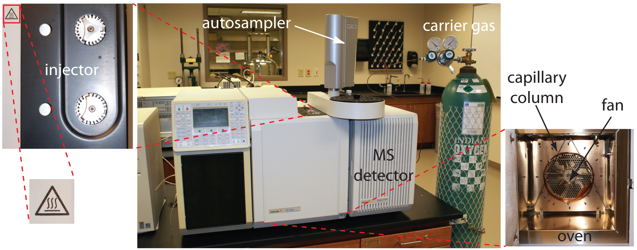
Figure 12.22 Example of a typical gas chromatograph with insets showing the heated injection ports—note the symbol indicating that it is hot—and the oven containing the column. This particular instrument is equipped with an autosampler for injecting samples, a capillary column, and a mass spectrometer (MS) as the detector. Note that the carrier gas is supplied by a tank of compressed gas.

12.4.1 Mobile Phase

The most common mobile phases for gas chromatography are He, Ar, and N₂, which have the advantage of being chemically inert toward both the sample and the stationary phase. The choice of carrier gas is often determined by the instrument’s detector. For a packed column the mobile phase velocity is usually 25–150 mL/min. The typical flow rate for a capillary column is 1–25 mL/min.

12.4.2 Chromatographic Columns

There are two broad classes of chromatographic columns: packed columns and capillary columns. In general, a packed column can handle larger samples and a capillary column can separate more complex mixtures.

Packed Columns

Packed columns are constructed from glass, stainless steel, copper, or aluminum, and are typically 2–6 m in length with internal diameters of 2–4 mm. The column is filled with a particulate solid support, with particle diameters ranging from 37–44 μm to 250–354 μm. Figure 12.23 shows a typical example of a packed column.

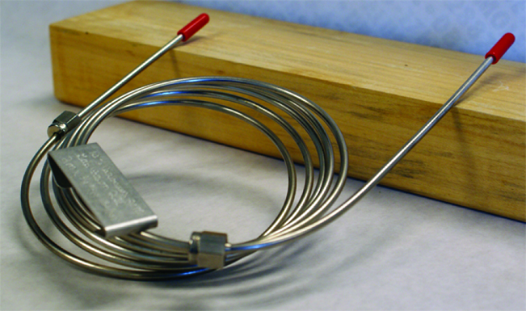
Figure 12.23 Typical example of a packed column for gas chromatography. This column is made from stainless steel and is 2 m long with an internal diameter of 3.2 mm. The packing material in this column has a particle diameter of 149–177 μm. To put this in perspective, beach sand has a typical diameter of 700 μm and the diameter of fine grained sand is 250 μm.

The most widely used particulate support is diatomaceous earth, which is composed of the silica skeletons of diatoms. These particles are very porous, with surface areas ranging from 0.5–7.5 m²/g, providing ample contact between the mobile phase and the stationary phase. When hydrolyzed, the surface of a diatomaceous earth contains silanol groups (–SiOH), which serve as active sites for absorbing solute molecules in gas-solid chromatography (GSC).

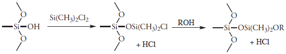
In gas-liquid chromatography (GLC), we coat the packing material with a liquid mobile phase. To prevent any uncoated packing material from adsorbing solutes, which degrades the quality of the separation, the surface silanols are deactivated by reacting them with dimethyldichlorosilane and rinsing with an alcohol—typically methanol—before coating the particles with stationary phase.

Other types of solid supports include glass beads and fluorocarbon polymers, which have the advantage of being more inert than diatomaceous earth.

To minimize the effect on plate height from multiple path and mass transfer, the diameter of the packing material should be as small as possible (see equation 12.21 and 12.25) and loaded with a thin film of stationary phase (see equation 12.23). Compared to capillary columns, which are discussed below, a packed column can handle larger sample volumes, typically 0.1–10 μL. Column efficiencies range from several hundred to 2000 plates/m, with a typical column having 3000–10 000 theoretical plates. The column in Figure 12.23, for example, has approximately 1800 plates/m, or a total of approximately 3600 theoretical plates. If we assume a V_max/V_min ≈ 50, then it has a peak capacity of

\[n_\ce{c}= 1 + \dfrac{\sqrt{3600}}{4}\ln(50) ≈ 60\]

Note

You can use equation 12.16 to estimate a column’s peak capacity.

Capillary Columns

A capillary, or open tubular column is constructed from fused silica and is coated with a protective polymer coating. Columns range from 15–100 m in length with an internal diameter of approximately 150–300 μm. Figure 12.24 shows a typical example of a capillary column.

Figure 12.24 Typical example of a capillary column for gas chromatography. This column is 30 m long with an internal diameter of 247 μm. The interior surface of the capillary has a 0.25 μm coating of the liquid phase.

Capillary columns are of three principle types. In a wall-coated open tubular column (WCOT) a thin layer of stationary phase, typically 0.25 μm thick, is coated on the capillary’s inner wall. In a porous-layer open tubular column (PLOT), a porous solid support—alumina, silica gel, and molecular sieves are typical examples—is attached to the capillary’s inner wall. A support-coated open tubular column (SCOT) is a PLOT column that includes a liquid stationary phase. Figure 12.25 shows the differences between these types of capillary columns.

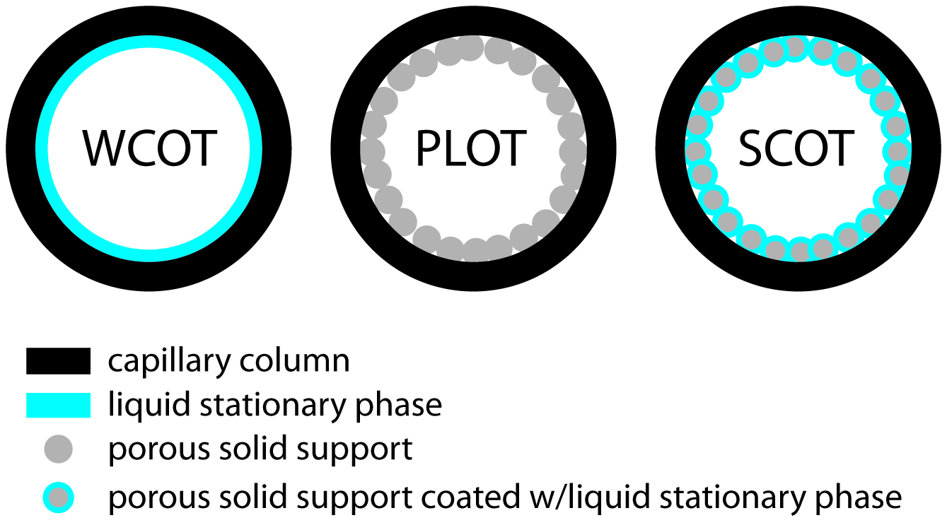
Figure 12.25 Cross-sections through the three types of capillary columns.

A capillary column provides a significant improvement in separation efficiency because it has more theoretical plates per meter and is longer than a packed column. For example, the capillary column in Figure 12.24 has almost 4300 plates/m, or a total of 129 000 theoretical plates. If we assume a V_max/V_min ≈ 50, then it has a peak capacity of approximately 350. On the other hand, a packed column can handle a larger sample. Because of its smaller diameter, a capillary column requires a smaller sample, typically less than 10^–2 μL.

Stationary Phases for Gas–Liquid Chromatography

Elution order in gas–liquid chromatography depends on two factors: the boiling point of the solutes, and the interaction between the solutes and the stationary phase. If a mixture’s components have significantly different boiling points, then the choice of stationary phase is less critical. If two solutes have similar boiling points, however, then a separation is possible only if the stationary phase selectively interacts with one of the solutes. As a general rule, nonpolar solutes are more easily separated with a nonpolar stationary phase, and polar solutes are easier to separate when using a polar stationary phase.

There are several important criteria for choosing a stationary phase: it must not react chemically with the solutes, it must be thermally stable, it must have a low volatility, and it must have a polarity that is appropriate for the sample’s components. Table 12.2 summarizes the properties of several popular stationary phases.

Table 12.2: Selected Examples of Stationary Phases for Gas–Liquid Chromatography

stationary phase	polarity	trade name	temperature limit (^oC)	representative applications
squalane	nonpolar	Squalane	150	low-boiling aliphatics hydrocarbons
Apezion L	nonpolar	Apezion L	300	amides, fatty acid methyl esters, terpenoids
polydimethyl siloxane	slightly polar	SE-30	300–350	alkaloids, amino acid derivatives, drugs, pesticides, phenols, steroids
phenylmethyl polysiloxane (50% phenyl, 50% methyl)	moderately polar	OV-17	375	alkaloids, drugs, pesticides, polyaromatic hydrocarbons, polychlorinated biphenyls
trifluoropropylmethyl polysiloxane (50% trifluoropropyl, 50% methyl)	moderately polar	OV-210	275	alkaloids, amino acid derivatives, drugs, halogenated compounds, ketones
cyanopropylphenylmethyl polysiloxane (50% cyanopropyl, 50% phenylmethyl)	polar	OV-225	275	nitriles, pesticides, steroids
polyethylene glycol	polar	Carbowax 20M	225	aldehydes, esters, ethers, phenols

Many stationary phases have the general structure shown in Figure 12.26a. A stationary phase of polydimethyl siloxane, in which all the –R groups are methyl groups, –CH₃, is nonpolar and often makes a good first choice for a new separation. The order of elution when using polydimethyl siloxane usually follows the boiling points of the solutes, with lower boiling solutes eluting first. Replacing some of the methyl groups with other substituents increases the stationary phase’s polarity and provides greater selectivity. For example, replacing 50% of the –CH₃ groups with phenyl groups, –C₆H₅, produces a slightly polar stationary phase. Increasing polarity is provided by substituting trifluoropropyl, –C₃H₆CF, and cyanopropyl, –C₃H₆CN, functional groups, or by using a stationary phase of polyethylene glycol (Figure 12.26b).

Figure 12.26: General structures of common stationary phases: (a) substituted polysiloxane; (b) polyethylene glycol.

An important problem with all liquid stationary phases is their tendency to elute, or bleed from the column when it is heated. The temperature limits in Table 12.2 minimize this loss of stationary phase. Capillary columns with bonded or cross-linked stationary phases provide superior stability. A bonded stationary phase is chemically attached to the capillary’s silica surface. Cross-linking, which is done after the stationary phase is in the capillary column, links together separate polymer chains, providing greater stability.

Another important consideration is the thickness of the stationary phase. From equation 12.23 we know that separation efficiency improves with thinner films of stationary phase. The most common thickness is 0.25 μm, although a thicker films may be used for highly volatile solutes, such as gases, because it has a greater capacity for retaining such solutes. Thinner films are used when separating low volatility solutes, such as steroids.

A few stationary phases take advantage of chemical selectivity. The most notable are stationary phases containing chiral functional groups, which can be used for separating enantiomers.⁷

12.4.3 Sample Introduction

Three considerations determine how we introduce a sample to the gas chromatograph. First, all of the sample’s constituents must be volatile. Second, the analytes must be present at an appropriate concentration. Finally, the physical process of injecting the sample must not degrade the separation.

Preparing a Volatile Sample

Not every sample can be injected directly into a gas chromatograph. To move through the column, the sample’s constituents must be volatile. A solute of low volatility may be retained by the column and continue to elute during the analysis of subsequent samples. A nonvolatile solute will condense at the top of the column, degrading the column’s performance.

We can separate a sample’s volatile analytes from its nonvolatile components using any of the extraction techniques described in Chapter 7. A liquid–liquid extraction of analytes from an aqueous matrix into methylene chloride or another organic solvent is a common choice. Solid-phase extractions also are used to remove a sample’s nonvolatile components.

An attractive approach to isolating analytes is a solid-phase microextraction (SPME). In one approach, which is illustrated in Figure 12.27, a fused-silica fiber is placed inside a syringe needle. The fiber, which is coated with a thin film of an adsorbent, such as polydimethyl siloxane, is lowered into the sample by depressing a plunger and is exposed to the sample for a predetermined time. After withdrawing the fiber into the needle, it is transferred to the gas chromatograph for analysis.

Figure 12.27 Schematic diagram of a solid-phase microextraction device.

Two additional methods for isolating volatile analytes are a purge-and-trap and headspace sampling. In a purge-and-trap (see Figure 7.25 in Chapter 7), we bubble an inert gas, such as He or N₂, through the sample, releasing—or purging—the volatile compounds. These compounds are carried by the purge gas through a trap containing an absorbent material, such as Tenax, where they are retained. Heating the trap and back-flushing with carrier gas transfers the volatile compounds to the gas chromatograph. In headspace sampling we place the sample in a closed vial with an overlying air space. After allowing time for the volatile analytes to equilibrate between the sample and the overlying air, we use a syringe to extract a portion of the vapor phase and inject it into the gas chromatograph. Alternatively, we can sample the headspace with an SPME.

Thermal desorption is a useful method for releasing volatile analytes from solids. We place a portion of the solid in a glass-lined, stainless steel tube. After purging with carrier gas to remove any O₂ that might be present, we heat the sample. Volatile analytes are swept from the tube by an inert gas and carried to the GC. Because volatilization is not a rapid process, the volatile analytes are often concentrated at the top of the column by cooling the column inlet below room temperature, a process known as cryogenic focusing. Once the volatilization is complete, the column inlet is rapidly heated, releasing the analytes to travel through the column.

The reason for removing O₂ is to prevent the sample from undergoing an oxidation reaction when it is heated.

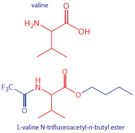
To analyze a nonvolatile analyte we must chemically convert it to a volatile form. For example, amino acids are not sufficiently volatile to analyze directly by gas chromatography. Reacting an amino acid with 1-butanol and acetyl chloride produces an esterfied amino acid. Subsequent treatment with trifluoroacetic acid gives the amino acid’s volatile N-trifluoroacetyl-n-butyl ester derivative.

Adjusting the Analyte’s Concentration

In an analyte’s concentration is too small to give an adequate signal, then it needs to be concentrated before injecting the sample into the gas chromatograph. A side benefit of many extraction methods is that they often concentrate the analytes. Volatile organic materials isolated from an aqueous sample by a purge-and-trap, for example, may be concentrated by as much as 1000×.

If an analyte is too concentrated it is easy to overload the column, resulting in peak fronting (see Figure 12.14 ) and a poor separation. In addition, the analyte’s concentration may exceed the detector’s linear response. Injecting less sample or diluting the sample with a volatile solvent, such as methylene chloride, are two possible solutions to this problem.

Injecting the Sample

In Section 12.3.3 we examined several explanations for why a solute’s band increases in width as it passes through the column, a process we called band broadening. We also introduce an additional source of band broadening if we fail to inject the sample into the minimum possible volume of mobile phase. There are two principal sources of this precolumn band broadening: injecting the sample into a moving stream of mobile phase and injecting a liquid sample instead of a gaseous sample. The design of a gas chromatograph’s injector helps minimize these problems.

An example of a simple injection port for a packed column is shown in Figure 12.28. The top of the column fits within a heated injector block, with carrier gas entering from the bottom. The sample is injected through a rubber septum using a microliter syringe such as the one shown in Figure 12.29. Injecting the sample directly into the column minimizes band broadening by mixing the sample with the smallest possible amount of carrier gas. The injector block is heated to a temperature that is at least 50^oC above the sample component with the highest boiling point, ensuring a rapid vaporization of the sample’s components.

Figure 12.28 Schematic diagram showing a heated GC injector port for use with packed columns. The needle pierces a rubber septum and enters into the top of the column, which is located within a heater block.

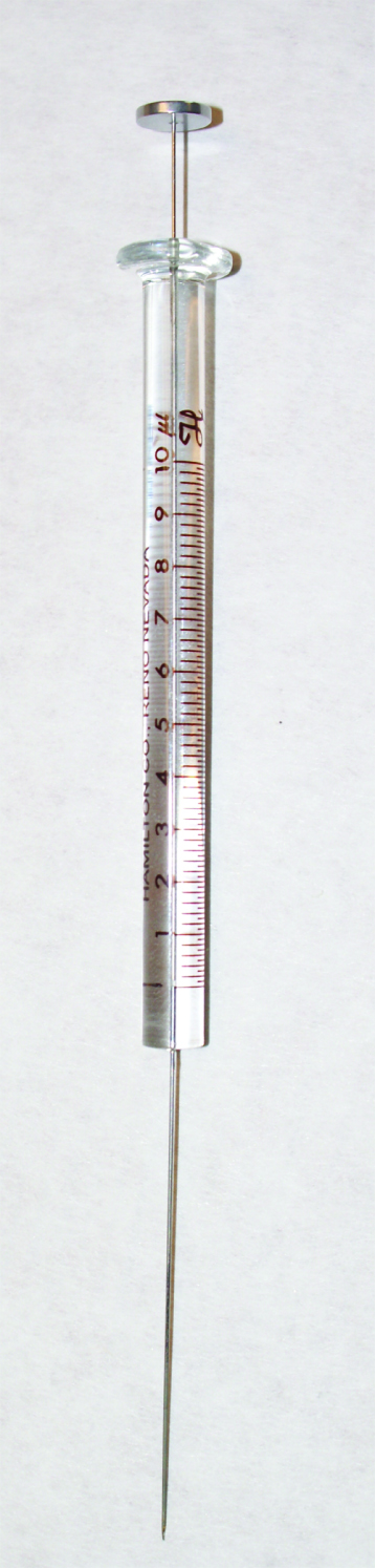
Figure 12.29 Example of a syringe for injecting samples into a gas chromatograph. This syringe has a maximum capacity of 10 μL with graduations every 0.1 μL.

Because a capillary column’s volume is significantly smaller than that for a packed column, it requires a different style of injector to avoid over-loading the column with sample. Figure 12.30 shows a schematic diagram of a typical split/splitless injector for use with capillary columns.

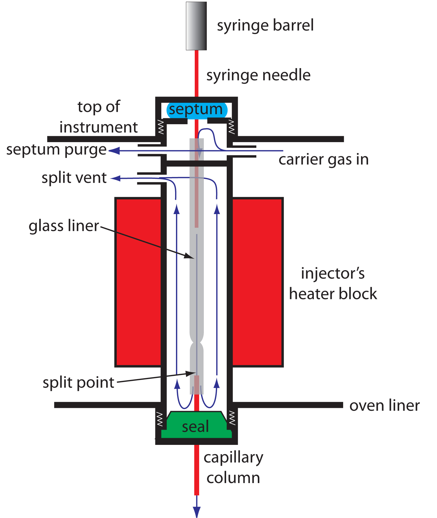
Figure 12.30 Schematic diagram showing a split/splitless injection port for use with capillary columns. The needle pierces a rubber septum and enters into a glass liner, which is located within a heater block. In a split injection the split vent is open; the split vent is closed for a splitless injection.

In a split injection we inject the sample through a rubber septum using a microliter syringe. Instead of injecting the sample directly into the column, it is injected into a glass liner where it mixes with the carrier gas. At the split point, a small fraction of the carrier gas and sample enters the capillary column with the remainder exiting through the split vent. By controlling the flow rate of the carrier gas entering the injector, and the flow rates through the septum purge and the split vent, we can control what fraction of the sample enters the capillary column, typically 0.1–10%.

For example, if the carrier gas flow rate is 50 mL/min, and the flow rates for the septum purge and the split vent are 2 mL/min and 47 mL/min, respectively, then the flow rate through the column is 1 mL/min (= 50 – 2 – 46). The ratio of sample entering the column is 1/50, or 2%.

In a splitless injection, which is useful for trace analysis, we close the split vent and allow all the carrier gas passing through the glass liner to enter the column—this allows virtually all the sample to enters the column. Because the flow rate through the injector is low, significant precolumn band broadening is a problem. Holding the column’s temperature approximately 20–25^oC below the solvent’s boiling point allows the solvent to condense at the entry to the capillary column, forming a barrier that traps the solutes. After allowing the solutes to concentrate, the column’s temperature is increased and the separation begins.

For samples that decompose easily, an on-column injection may be necessary. In this method the sample is injected directly into the column without heating. The column temperature is then increased, volatilizing the sample with as low a temperature as is practical.

12.4.4 Temperature Control

Control of the column’s temperature is critical to attaining a good separation in gas chromatography. For this reason the column is placed inside a thermostated oven (see Figure 12.22). In an isothermal separation we maintain the column at a constant temperature. To increase the interaction between the solutes and the stationary phase, the temperature usually is set slightly below that of the lowest-boiling solute.

One difficulty with an isothermal separation is that a temperature favoring the separation of a low-boiling solute may lead to an unacceptably long retention time for a higher-boiling solute. Temperature programming provide a solution to this problem. At the beginning of the analysis we set the column’s initial temperature below that for the lowest-boiling solute. As the separation progresses, we slowly increase the temperature at either a uniform rate or in a series of steps.

You may recall that we called this the general elution problem (see Figure 12.16).

12.4.5 Detectors for Gas Chromatography

The final part of a gas chromatograph is the detector. The ideal detector has several desirable features, including: a low detection limit, a linear response over a wide range of solute concentrations (which makes quantitative work easier), sensitivity for all solutes or selectivity for a specific class of solutes, and an insensitivity to a change in flow rate or temperature.

Thermal Conductivity Detector (TCD)

One of the earliest gas chromatography detectors takes advantage of the mobile phase’s thermal conductivity. As the mobile phase exits the column it passes over a tungsten-rhenium wire filament (see Figure 12.31). The filament’s electrical resistance depends on its temperature, which, in turn, depends on the thermal conductivity of the mobile phase. Because of its high thermal conductivity, helium is the mobile phase of choice when using a thermal conductivity detector (TCD).

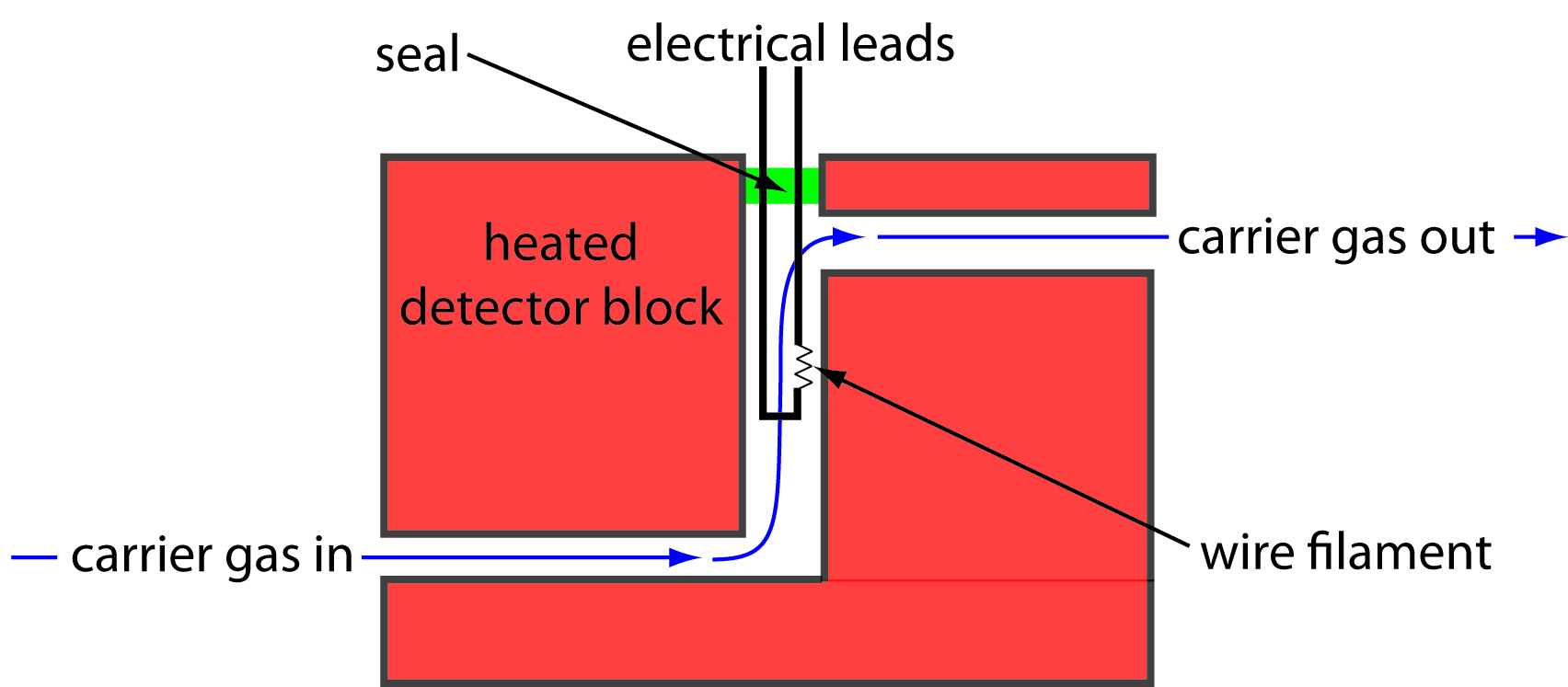
Figure 12.31 Schematic diagram showing a thermal conductivity detector. This is one cell of a matched pair. The sample cell takes the carrier gas as it elutes from the column. A source of carrier gas that bypasses the column passes through a reference cell.

When a solute elutes from the column, the thermal conductivity of the mobile phase in the TCD cell decreases and the temperature of the wire filament, and thus it resistance, increases. A reference cell, through which only the mobile phase passes, corrects for any time-dependent variations in flow rate, pressure, or electrical power, all of which may lead to a change in the filament’s resistance.

Because all solutes affect the mobile phase’s thermal conductivity, the thermal conductivity detector is a universal detector. Another advantage is the TCD’s linear response over a concentration range spanning 10⁴–10⁵ orders of magnitude. The detector also is non-destructive, allowing us to isolate analytes using a postdetector cold trap. One significant disadvantage of the TCD detector is its poor detection limit for most analytes.

Flame Ionization Detector (FID)

The combustion of an organic compound in an H₂/air flame results in a flame containing electrons and organic cations, presumably CHO⁺. Applying a potential of approximately 300 volts across the flame creates a small current of roughly 10^–9 to 10^–12 amps. When amplified, this current provides a useful analytical signal. This is the basis of the popular flame ionization detector, a schematic diagram of which is shown in Figure 12.32.

Figure 12.32 Schematic diagram showing a flame ionization detector. The eluent from the column mixes with H₂ and is burned in the presence of excess air. Combustion produces a flame containing electrons and the cation CHO⁺. Applying a potential between the flame tip and the collector, a current that is proportional to the concentration of cations in the flame.

Most carbon atoms—except those in carbonyl and carboxylic groups—generate a signal, which makes the FID an almost universal detector for organic compounds. Most inorganic compounds and many gases, such as H₂O and CO₂, are not detected, which makes the FID detector a useful detector for the analysis of atmospheric and aqueous environmental samples. Advantages of the FID include a detection limit that is approximately two to three orders of magnitude smaller than that for a thermal conductivity detector, and a linear response over 10⁶–10⁷ orders of magnitude in the amount of analyte injected. The sample, of course, is destroyed when using a flame ionization detector.

Electron Capture Detector (ECD)

The electron capture detector is an example of a selective detector. As shown in Figure 12.33, the detector consists of a β-emitter, such as ⁶³Ni. The emitted electrons ionize the mobile phase, which is usually N₂, generating a standing current between a pair of electrodes. When a solute with a high affinity for capturing electrons elutes from the column, the current decreases. This decrease in current serves as the signal. The ECD is highly selective toward solutes with electronegative functional groups, such as halogens and nitro groups, and is relatively insensitive to amines, alcohols, and hydrocarbons. Although its detection limit is excellent, its linear range extends over only about two orders of magnitude.

A β-particle is an electron.

Figure 12.33 Schematic diagram showing an electron capture detector.

Mass Spectrometer (MS)

A mass spectrometer is an instrument that ionizes a gaseous molecule using enough energy that the resulting ion breaks apart into smaller ions. Because these ions have different mass-to-charge ratios, it is possible to separate them using a magnetic field or an electrical field. The resulting mass spectrum contains both quantitative and qualitative information about the analyte. Figure 12.34 shows a mass spectrum for toluene.

Figure 12.34 Mass spectrum for toluene highlighting the molecular ion in green (m/z = 92), and two fragment ions in blue (m/z = 91) and in red (m/z = 65). A mass spectrum provides both quantitative and qualitative information: the height of any peak is proportional to the amount of toluene in the mass spectrometer and the fragmentation pattern is unique to toluene.

Figure 12.35 shows a block diagram of a typical gas chromatography-mass spectrometer (GC–MS) instrument. The effluent from the column enters the mass spectrometer’s ion source in a manner that eliminates the majority of the carrier gas. In the ionization chamber the remaining molecules—a mixture of carrier gas, solvent, and solutes—undergo ionization and fragmentation. The mass spectrometer’s mass analyzer separates the ions by their mass-to-charge ratio. A detector counts the ions and displays the mass spectrum.

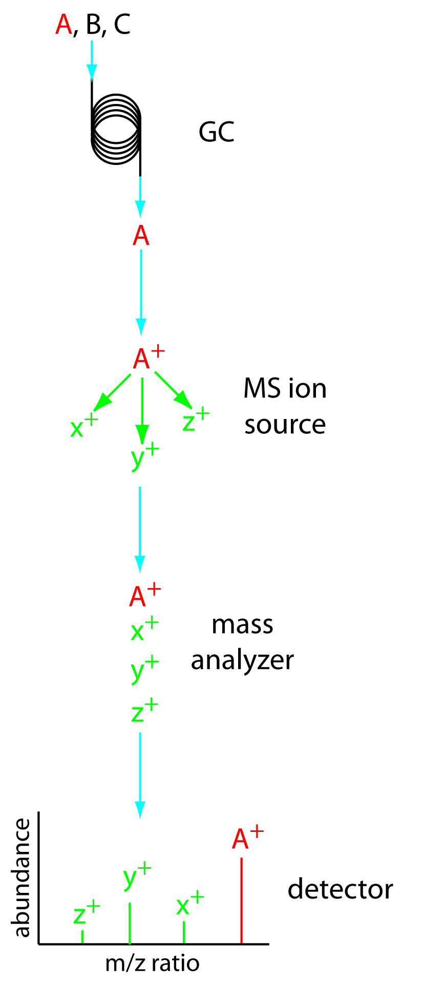
Figure 12.35 Block diagram of GC–MS. A three component mixture enters the GC. When component A elutes from the column, it enters the MS ion source and ionizes to form the parent ion and several fragment ions. The ions enter the mass analyzer, which separates them by their mass-tocharge ratio, providing the mass spectrum shown at the detector.

There are several options for monitoring the chromatogram when using a mass spectrometer as the detector. The most common method is to continuously scan the entire mass spectrum and report the total signal for all ions reaching the detector during each scan. This total ion scan provides universal detection for all analytes. We can achieve some degree of selectivity by monitoring only specific mass-to-charge ratios, a process called selective-ion monitoring. A mass spectrometer provides excellent detection limits, typically 25 fg to 100 pg, with a linear range of 10⁵ orders of magnitude. Because we are continuously recording the mass spectrum of the column’s eluent, we can go back and examine the mass spectrum for any time increment. This is a distinct advantage for GC–MS because we can use the mass spectrum to help identify a mixture’s components.

Other Detectors

Two additional detectors are similar in design to a flame ionization detector. In the flame photometric detector optical emission from phosphorous and sulfur provides a detector selective for compounds containing these elements. The thermionic detector responds to compounds containing nitrogen or phosphorous.

A Fourier transform infrared spectrophotometer (FT–IR) also can serve as a detector. In GC–FT–IR, effluent from the column flows through an optical cell constructed from a 10–40 cm Pyrex tube with an internal diameter of 1–3 mm. The cell’s interior surface is coated with a reflecting layer of gold. Multiple reflections of the source radiation as it is transmitted through the cell increase the optical path length through the sample. As is the case with GC–MS, an FT–IR detector continuously records the column eluent’s spectrum, which allows us to examine the IR spectrum for any time increment.

Note

See Chapter 10.3 for a discussion of FT-IR spectroscopy and instrumentation.

12.4.6 Quantitative Applications

Gas chromatography is widely used for the analysis of a diverse array of samples in environmental, clinical, pharmaceutical, biochemical, forensic, food science and petrochemical laboratories. Table 12.3 provides some representative examples of applications.

Table 12.3 Representative Applications of Gas Chromatography

area	applications
environmental analysis	green house gases (CO2, CH4, NOx) in air pesticides in water, wastewater, and soil vehicle emissions trihalomethanes in drinking water
clinical analysis	drugs blood alcohols
forensic analysis	analysis of arson accelerants detection of explosives
consumer products	volatile organics in spices and fragrances trace organics in whiskey monomers in latex paint
petroleum and chemical industry	purity of solvents refinery gas composition of gasoline

Quantitative Calculations

In a GC analysis the area under the peak is proportional to the amount of analyte injected onto the column. The peak’s area is determined by integration, which usually is handled by the instrument’s computer or by an electronic integrating recorder. If two peak are fully resolved, the determination of their respective areas is straightforward. Overlapping peaks, however, require a choice between one of several options for dividing up the area shared by the two peaks (Figure 12.36). Which method to use depends on the relative size of the two peaks and their resolution. In some cases, the use of peak heights provides more accurate results.⁸

Before electronic integrating recorders and computers, two methods were used to find the area under a curve. One method used a manual planimeter; as you use the planimeter to trace an object’s perimeter, it records the area. A second approach for finding the area is the cut-and-weigh method. The chromatogram is recorded on a piece of paper. Each peak of interest is cut out and weighed. Assuming the paper is uniform in thickness and density of fibers, the ratio of weights for two peaks is the same as the ratio of areas. Of course, this approach destroys your chromatogram.

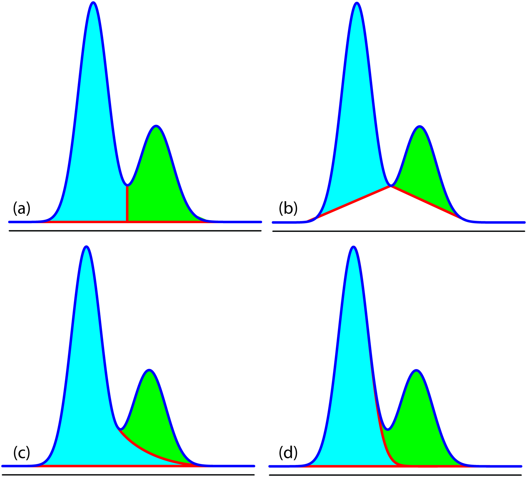
Figure 12.36 Four methods for determining the areas under two overlapping chromatographic peaks: (a) the drop method; (b) the valley method; (c) the exponential skim method; and (d) the Gaussian skim method. Other methods for determining areas also are available.

For quantitative work we need to establish a calibration curve that relates the detector’s response to the concentration of analyte. If the injection volume is identical for every standard and sample, then an external standardization provides both accurate and precise results. Unfortunately, even under the best conditions the relative precision for replicate injections may differ by 5%—often it is substantially worse. For quantitative work requiring high accuracy and precision, the use of internal standards is recommended.

Note

To review the method of internal standards, see Section 5.3.4.

Example 12.5

Marriott and Carpenter report the following data for five replicate injections of a mixture consisting of 1% v/v methylisobutylketone and 1% v/v p-xylene in dichloromethane.⁹

injection	peak	peak area (arb. units)
I	1	49075
	2	78112
II	1	85829
	2	135404
III	1	84136
	2	132332
IV	1	71681
	2	112889
V	1	58054
	2	91287

Assume that p-xylene (peak 2) is the analyte, and that methylisobutylketone (peak 1) is the internal standard. Determine the 95% confidence interval for a single-point standardization, with and without using the internal standard.

Solution

For a single-point external standardization we ignore the internal standard and determine the relationship between the peak area for p-xylene, A₂, and the concentration, C₂, of p-xylene.

\[A_2 = kC_2\]

Substituting the known concentration for p-xylene and the appropriate peak areas, gives the following values for the constant k.

78 112 135 404 132 332 112 889 91 287

The average value for k is 110 000 with a standard deviation of 25 100 (a relative standard deviation of 22.8%). The 95% confidence interval is

\[\mu = \overline{X} ± \dfrac{ts}{\sqrt{n}} = 111000 ± \dfrac{(2.78)(25100)}{\sqrt{5}} = 111000 ± 31200\]

For an internal standardization, the relationship between the analyte’s peak area, A₂, the peak area for the internal standard, A₁, and their respective concentrations, C₂ and C₁, is

\[\dfrac{A_2}{A_1} = k\dfrac{C_2}{C_1}\]

Substituting the known concentrations and the appropriate peak areas gives the following values for the constant k.

1.5917 1.5776 1.5728 1.5749 1.5724

The average value for k is 1.5779 with a standard deviation of 0.0080 (a relative standard deviation of 0.507%). The 95% confidence interval is

\[\mu = \overline{X} ± \dfrac{ts}{\sqrt{n}} = 1.5779 ± \dfrac{(2.78)(0.0080)}{\sqrt{5}} = 1.5779 ± 0.0099\]

Although there is a substantial variation in the individual peak areas for this set of replicate injections, the internal standard compensates for these variations, providing a more accurate and precise calibration.

Practice Exercise 12.5

Figure 12.37 shows chromatograms for five standards and one sample. Each standard and the sample contains the same concentration of an internal standard, which is 2.50 mg/mL. For the five standards, the concentrations of analyte are 0.20 mg/mL, 0.40 mg/mL, 0.60 mg/mL, 0.80 mg/mL, and 1.00 mg/mL, respectively. Determine the concentration of analyte in the sample by (a) ignoring the internal standards and creating an external standards calibration curve, and (b) creating an internal standard calibration curve. For each approach, report the analyte’s concentration and the 95% confidence interval. Use peak heights instead of peak areas.

(You may wish to review our earlier coverage of linear regression in Chapter 5.4.)

Click here to review your answer to this exercise.

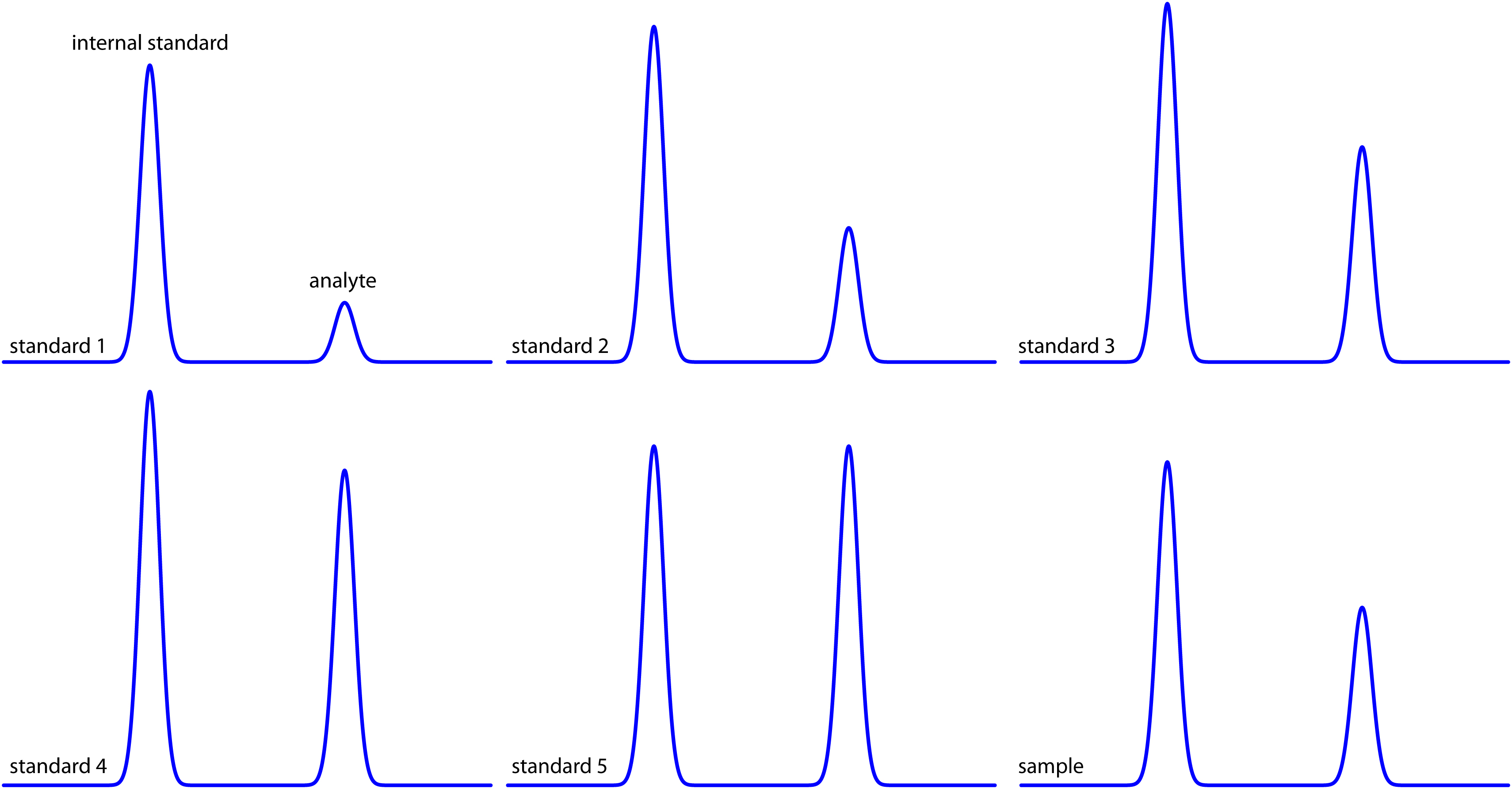
Figure 12.37 Chromatograms for Practice Exercise 12.5.

12.4.7 Qualitative Applications

In addition to a quantitative analysis, we also can use chromatography to identify the components of a mixture. As noted earlier, when using an FT–IR or a mass spectrometer as the detector we have access to the eluent’s full spectrum for any retention time. By interpreting the spectrum or by searching against a library of spectra, we can identify the analyte responsible for each chromatographic peak.

In addition to identifying the component responsible for a particular chromatographic peak, we also can use the saved spectra to evaluate peak purity. If only one component is responsible for a chromatographic peak, then the spectra should be identical throughout the peak’s elution. If a spectrum at the beginning of the peak’s elution is different from a spectrum taken near the end of the peak’s elution, then there must be at least two components that are co-eluting.

When using a nonspectroscopic detector, such as a flame ionization detector, we must find another approach if we need to identify the components of a mixture. One approach is to spike the sample the suspected compound and looking for an increase in peak height. We also can compare a peak’s retention time to the retention time for a known compound if we use identical operating conditions.

Because a compound’s retention times on two identical columns are not likely to be the same—differences in packing efficiency, for example, will affect a solute’s retention time on a packed column—a table of standard retention times is not useful. Kovat’s retention index provides one solution to the problem of matching retention times. Under isothermal conditions, the adjusted retention times for normal alkanes increase logarithmically. Kovat defined the retention index, I, for a normal alkane as 100 times the number of carbon atoms. For example, the retention index is 400 for butane, C₄H₁₀, and 500 for pentane, C₅H₁₂. To determine the a compound’s retention index, I_cpd, we use the following formula

\[I_\textrm{cpd} = 100 × \dfrac{\log t^′_\textrm{r,cpd} - \log t^′_{\textrm{r,}x}}{\log t^′_{\textrm{r,}x+1} - \log t^′_{\textrm{r,}x}} + I_x\tag{12.27}\]

where t′_r,cpd is the compound’s adjusted retention time, t′_x,r and t′_x,r+1 are the adjusted retention times for the normal alkanes that elute immediately before the compound and after the compound, respectively, and I_x is the retention index for the normal alkane eluting immediately before the compound. A compound’s retention index for a particular set of chromatographic conditions—stationary phase, mobile phase, column type, column length, temperature, etc.—should be reasonably consistent from day to day and between different columns and instruments.

Tables of Kovat’s retention indices are available; see, for example, the NIST Chemistry Webbook. A search for toluene returns 341 values of I for over 20 different stationary phases, and for both packed columns and capillary columns.

Example 12.6

In a separation of a mixture of hydrocarbons the following adjusted retention times were measured: 2.23 min for propane, 5.71 min for isobutane, and 6.67 min for butane. What is the Kovat’s retention index for each of these hydrocarbons?

Solution

Kovat’s retention index for a normal alkane is 100 times the number of carbons; thus, for propane, I = 300 and for butane, I = 400. To find Kovat’s retention index for isobutane we use equation 12.27.

\[I_\textrm{cpd}= 100 × \dfrac{\log(5.71) - \log(2.23)}{\log(6.67) - \log(2.23)} + 300 = 386\]

Practice Exercise 12.6

When using a column with the same stationary phase as in Example 12.6, you find that the retention times for propane and butane are 4.78 min and 6.86 min, respectively. What is the expected retention time for isobutane?

Click here to review your answer to this exercise.

Note

The best way to appreciate the theoretical and practical details discussed in this section is to carefully examine a typical analytical method. Although each method is unique, the following description of the determination of trihalomethanes in drinking water provides an instructive example of a typical procedure. The description here is based on a Method 6232B in Standard Methods for the Examination of Water and Wastewater, 20th Ed., American Public Health Association: Washington, DC, 1998.

Representative Method 12.1: Determination of Trihalomethanes in Drinking Water

Description of Method

Trihalomethanes, such as chloroform, CHCl₃, and bromoform, CHBr₃, are found in most chlorinated waters. Because chloroform is a suspected carcinogen, the determination of trihalomethanes in public drinking water supplies is of considerable importance. In this method the trihalomethanes CHCl₃, CHBrCl₂, CHBr₂Cl, and CHBr₃ are isolated using a liquid–liquid extraction with pentane and determined using a gas chromatograph equipped with an electron capture detector.

Procedure

Collect the sample in a 40-mL glass vial with a screw-cap lined with a TFE-faced septum. Fill the vial to overflowing, ensuring that there are no air bubbles. Add 25 mg of ascorbic acid as a reducing agent to quench the further production of trihalomethanes. Seal the vial and store the sample at 4^oC for no longer than 14 days.

(TFE is tetrafluoroethylene. Teflon is a polymer formed from TFE.)

Prepare a standard stock solution for each trihalomethane by placing 9.8 mL of methanol in a 10-mL volumetric flask. Let the flask stand for 10 min, or until all surfaces wetted with methanol are dry. Weigh the flask to the nearest ±0.1 mg. Using a 100-μL syringe, add 2 or more drops of trihalomethane to the volumetric flask, allowing each drop to fall directly into the methanol. Reweigh the flask before diluting to volume and mixing. Transfer the solution to a 40-mL glass vial with a TFE-lined screw-top and report the concentration in μg/mL. Store the stock solutions at –10 to –20^oC and away from the light.

Prepare a multicomponent working standard from the stock standards by making appropriate dilutions of the stock solution with methanol in a volumetric flask. Choose concentrations so that calibration standards (see below) require no more than 20 μL of working standard per 100 mL of water.

Using the multicomponent working standard, prepare at least three, but preferably 5–7 calibration standards. At least one standard must be near the detection limit and the standards must bracket the expected concentration of trihalomethanes in the samples. Using an appropriate volumetric flask, prepare the standards by injecting at least 10 μL of the working standard below the surface of the water and dilute to volume. Mix each standard gently three times only. Discard the solution in the neck of the volumetric flask and then transfer the remaining solution to a 40-mL glass vial with a TFE-lined screw-top. If the standard has a headspace, it must be analyzed within 1 hr; standards without any headspace may be held for up to 24 hr.

Prepare an internal standard by dissolving 1,2-dibromopentane in hexane. Add a sufficient amount of this solution to pentane to give a final concentration of 30 μg 1,2-dibromopentane/L.

To prepare the calibration standards and samples for analysis, open the screw top vial and remove 5 mL of the solution. Recap the vial and weigh to the nearest ±0.1 mg. Add 2.00 mL of pentane (with the internal standard) to each vial and shake vigorously for 1 min. Allow the two phases to separate for 2 min and then use a glass pipet to transfer at least 1 mL of the pentane (the upper phase) to a 1.8-mL screw top sample vial with a TFE septum, and store at 4^oC until you are ready to inject them into the GC. After emptying, rinsing, and drying the sample’s original vial, weigh it to the nearest ±0.1 mg and calculate the sample’s weight to ±0.1 g. If the density is 1.0 g/mL, then the sample’s weight is equivalent to its volume.

Inject a 1–5 μL aliquot of the pentane extracts into a GC equipped with a 2-mm ID, 2-m long glass column packed with a stationary phase of 10% squalane on a packing material of 80/100 mesh Chromosorb WAW. Operate the column at 67^oC and a flow rate of 25 mL/min.

(A variety of other columns can be used. Another option, for example, is a 30-m fused silica column with an internal diameter of 0.32 mm and a 1 μm coating of the stationary phase DB-1. A linear flow rate of 20 cm/s is used with the following temperature program: hold for 5 min at 35^oC; increase to 70^oC at 10^oC/min; increase to 200^oC at 20^oC.)

Questions

1. A simple liquid–liquid extraction rarely extracts 100% of the analyte. How does this method account for incomplete extractions?

Because the extraction procedure for the samples and the standards are identical, the ratio of analyte between any two samples or standards is unaffected by an incomplete extraction.

2. Water samples are likely to contain trace amounts of other organic compounds, many of which will extract into pentane along with the trihalomethanes. A short, packed column, such as the one used in this method, generally does not do a particularly good job of resolving chromatographic peaks. Why do we not need to worry about these other compounds?

An electron capture detector responds only to compounds, such as the trihalomethanes, that have electronegative functional groups. Because an electron capture detector will not respond to most of the potential interfering compounds, the chromatogram will have relatively few peaks other than those for the trihalomethanes and the internal standard.

3. Predict the order in which the four analytes elute from the GC column.

Retention time should follow the compound’s boiling points, eluting from the lowest boiling point to the highest boiling points. The elution order is CHCl₃ (61.2^oC), CHCl₂Br (90^oC), CHClBr₂ (119^oC), and CHBr₃ (149.1^oC).

4. Although chloroform is an analyte, it also is an interferent because it is present at trace levels in the air. Any chloroform present in the laboratory air, for example, may enter the sample by diffusing through the sample vial’s silicon septum. How can we determine whether samples have been contaminated in this manner?

A sample blank of trihalomethane-free water can be kept with the samples at all times. If the sample blank shows no evidence for chloroform, then we can safely assume that the samples also are free from contamination.

5. Why is it necessary to collect samples without any headspace (a layer of air overlying the liquid) in the sample vial?

Because trihalomethanes are volatile, the presence of a headspace allows for the possible loss of analyte.

6. In preparing the stock solution for each trihalomethane, the procedure specifies that we can add the two or more drops of the pure compound by dropping them into the volumetric flask containing methanol. When preparing the calibration standards, however, the working standard must be injected below the surface of the water. Explain the reason for this difference.

When preparing a stock solution, the potential loss of the volatile trihalomethane is unimportant because we determine its concentration by weight after adding it to the water. When we prepare the calibration standard, however, we must ensure that the addition of trihalomethane is quantitative.

12.4.8 Evaluation

Scale of Operation

Gas chromatography is used to analyze analytes present at levels ranging from major to ultratrace components. Depending on the detector, samples with major and minor analytes may need to be diluted before analysis. The thermal conductivity and flame ionization detectors can handle larger amounts of analyte; other detectors, such as an electron capture detector or a mass spectrometer, require substantially smaller amounts of analyte. Although the injection volume for gas chromatography is quite small—typically about a microliter—the amount of available sample must be sufficient that the injection is a representative subsample. For a trace analyte, the actual amount of injected analyte is often in the picogram range. Using Representative Method 12.1 as an example, a 3.0-μL injection of 1 μg/L CHCl₃ is equivalent to 15 pg of CHCl₃, assuming a 100% extraction efficiency.

See Figure 3.5 to review the meaning of major, minor, and ultratrace analytes.

Accuracy

The accuracy of a gas chromatographic method varies substantially from sample to sample. For routine samples, accuracies of 1–5% are common. For analytes present at very low concentration levels, samples with complex matrices, or samples requiring significant processing before analysis, accuracy may be substantially poorer. In the analysis for trihalomethanes described in Representative Method 12.1, for example, determinate errors as large as ±25% are possible.

Precision

The precision of a gas chromatographic analysis includes contributions from sampling, sample preparation, and the instrument. The relative standard deviation due to the instrument is typically 1–5%, although it can be significantly higher. The principle limitations are detector noise, which affects the determination of peak area, and the reproducibility of injection volumes. In quantitative work, the use of an internal standard compensates for any variability in injection volumes.

Sensitivity

In a gas chromatographic analysis, sensitivity is determined by the detector’s characteristics. Of particular importance for quantitative work is the detector’s linear range; that is, the range of concentrations over which a calibration curve is linear. Detectors with a wide linear range, such as the thermal conductivity detector and the flame ionization detector, can be used to analyze samples over a wide range of concentrations without adjusting operating conditions. Other detectors, such as the electron capture detector, have a much narrower linear range.

Selectivity

Because it combines separation with analysis, chromatographic methods provide excellent selectivity. By adjusting conditions it is usually possible to design a separation so that the analytes elute by themselves, even when the mixture is complex. Additional selectivity is obtained by using a detector, such as the electron capture detector, that does not respond to all compounds.

Time, Cost, and Equipment

Analysis time can vary from several minutes for samples containing only a few constituents, to more than an hour for more complex samples. Preliminary sample preparation may substantially increase the analysis time. Instrumentation for gas chromatography ranges in price from inexpensive (a few thousand dollars) to expensive (>$50,000). The more expensive models are equipped for capillary columns, include a variety of injection options and more sophisticated detectors, such as a mass spectrometer. Packed columns typically cost <$200, and the cost of a capillary column is typically $300–$1000.

Contributors

David Harvey (DePauw University)