
7.6: Classifying Separation Techniques
- Page ID
- 5572

We can separate an analyte and an interferent if there is a significant difference in at least one of their chemical or physical properties. Table 7.4 provides a partial list of separation techniques, classified by the chemical or physical property being exploited.
| Basis of Separation | Separation Technique |
|---|---|
| size | filtration dialysis size-exclusion chromatography |
| mass or density | centrifugation |
| complex formation | masking |
| change in physical state | distillation sublimation recrystallization |
| change in chemical state | precipitation electrodeposition volatilization |
| partitioning between phases | extraction chromatography |
7.6.1 Separations Based on Size
Size is the simplest physical property we can exploit in a separation. To accomplish the separation we use a porous medium through which only the analyte or the interferent can pass. Examples of size-based separations include filtration, dialysis, and size-exclusion. In a filtration we separate a particulate interferent from dissolved analytes using a filter whose pore size retains the interferent. The solution passing through the filter is called the filtrate, and the material retained by the filter is the retentate. Gravity filtration and suction filtration using filter paper are techniques with which you should already be familiar. Membrane filters, available in a variety of micrometer pores sizes, are the method of choice for particulates that are too small to be retained by filter paper. Figure 7.13 provides information about three types of membrane filters.
For applications of gravity filtration and suction filtration in gravimetric methods of analysis, see Chapter 8.
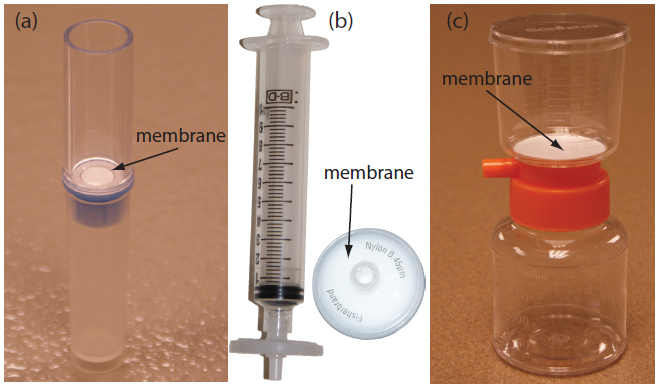
Figure 7.13: Three types of membrane filters for separating analytes from interferents. (a) A centrifugal filter for concentrating and desalting macromolecular solutions. The membrane has a nominal molecular weight cut-off of 1 × 10⁶ g/mol. The sample is placed in the upper reservoir and the unit is placed in a centrifuge. Upon spinning the unit at 2000×g–5000×g, the filtrate collects in the bottom reservoir and the retentate remains in the upper reservoir. (b) A 0.45 μm membrane syringe filter. The photo on the right shows the membrane filter in its casing. In the photo on the left, the filter is attached to a syringe. Samples are placed in the syringe and pushed through the filter. The filtrate is collected in a test tube or other suitable container. (c) A disposable filter system with a 0.22 μm cellulose acetate membrane filter. The sample is added to the upper unit and vacuum suction is used to draw the filtrate through the membrane and into the lower unit. To store the filtrate, the top half of the unit is removed and a cap placed on the lower unit. The filter unit shown here has a capacity of 150 mL.
Dialysis is another example of a separation technique that uses size to separate the analyte and the interferent. A dialysis membrane is usually constructed from cellulose and fashioned into tubing, bags, or cassettes. Figure 7.14 shows an example of a commercially available dialysis cassette. The sample is injected into the dialysis membrane, which is sealed tightly by a gasket, and the unit is placed in a container filled with a solution whose composition is different from the sample. If the concentration of a particular species is different on the membrane’s two sides, the resulting concentration gradient provides a driving force for its diffusion across the membrane. While small species freely pass through the membrane, larger species are unable to pass. Dialysis is frequently used to purify proteins, hormones, and enzymes. During kidney dialysis, metabolic waste products, such as urea, uric acid, and creatinine, are removed from blood by passing it over a dialysis membrane.
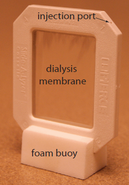
Figure 7.14: Example of a dialysis cassette. The dialysis membrane in this unit has a molecular weight cut-off of 10 000 g/mol. Two sheets of the membrane are separated by a gasket and held in place by the plastic frame. Four ports, one of which is labeled, provide a means for injecting the sample between the dialysis membranes. The cassette is inverted and submerged in a beaker containing the external solution, which is stirred using a stir bar. A foam buoy, used as a stand in the photo, serves as a float so that the unit remains suspended above the stir bar. The external solution is usually replaced several time during dialysis. When dialysis is complete, the solution remaining in the cassette is removed through an injection port.
Size-exclusion chromatography is a third example of a separation technique that uses size as a means for effecting a separation. In this technique a column is packed with small, approximately 10-μm, porous polymer beads of cross-linked dextrin or polyacrylamide. The pore size of the particles is controlled by the degree of cross-linking, with more cross-linking producing smaller pore sizes. The sample is placed into a stream of solvent that is pumped through the column at a fixed flow rate. Those species too large to enter the pores pass through the column at the same rate as the solvent. Species entering into the pores take longer to pass through the column, with smaller species needing more time to pass through the column. Size-exclusion chromatography is widely used in the analysis of polymers, and in biochemistry, where it is used for the separation of proteins.
Note
A more detailed treatment of size-exclusion chromatography, which also is called gel permeation chromatography, is in Chapter 12.
7.6.2 Separations Based on Mass or Density
If the analyte and the interferent differ in mass or density, then a separation using centrifugation may be possible. The sample is placed in a centrifuge tube and spun at a high angular velocity, measured in revolutions per minute (rpm). The sample’s constituents experience a centrifugal force that pulls them toward the bottom of the centrifuge tube. The species experiencing the greatest centrifugal force has the fastest sedimentation rate, and is the first to reach the bottom of the centrifuge tube. If two species have equal density, their separation is based on mass, with the heavier species having the greater sedimentation rate. If the species are of equal mass, then the species with the largest density has the greatest sedimentation rate.
Centrifugation is an important separation technique in biochemistry. Table 7.5, for example, lists conditions for separating selected cellular components. We can separate lysosomes from other cellular components by several differential centrifugations, in which we divide the sample into a solid residue and a supernatant solution. After destroying the cells, the solution is centrifuged at 15 000 × g (a centrifugal force that is 15 000 times that of the earth’s gravitational force) for 20 minutes, leaving a solid residue of cell membranes and mitochondria. The supernatant, which contains the lysosomes, is isolated by decanting it from the residue and centrifuged at 30 000 × g for 30 minutes, leaving a solid residue of lysosomes. Figure 7.15 shows a typical centrifuge capable of produce the centrifugal forces needed for biochemical separations.
| Components | Centrifugal Force (×g) | Time (min) |
|---|---|---|
| eukaryotic cells | 1000 | 5 |
| cell membranes, nuclei | 4000 | 10 |
| mitochondria, bacterial cells | 15000 | 20 |
| lysosomes, bacterial membranes | 30000 | 30 |
| ribosomes | 100000 | 180 |
Source: Adapted from Zubay, G. Biochemistry, 2nd ed. Macmillan: New York, 1988, p.120.
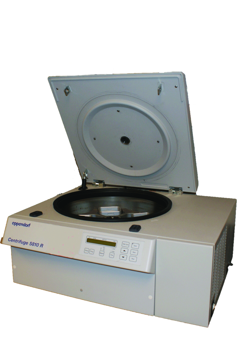
Figure 7.15: Bench-top centrifuge capable of reaching speeds up to 14 000 rpm and centrifugal forces of 20 800 × g. This particular centrifuge is refrigerated, allowing samples to be cooled to temperatures as low as –4oC.
An alternative approach to differential centrifugation is density gradient centrifugation. To prepare a sucrose density gradient, for example, a solution with a smaller concentration of sucrose—and, thus, of lower density—is gently layered upon a solution with a higher concentration of sucrose. Repeating this process several times, fills the centrifuge tube with a multi-layer density gradient. The sample is placed on top of the density gradient and centrifuged using a force greater than 150 000 × g. During centrifugation, each of the sample’s components moves through the gradient until it reaches a position where its density matches the surrounding sucrose solution. Each component is isolated as a separate band positioned where its density is equal to that of the local density within the gradient. Figure 7.16 provides an example of a typical sucrose density centrifugation for separating plant thylakoid membranes.

Figure 7.16: Example of a sucrose density gradient centrifugation of thylakoid membranes from wild type (WT) and lut2 plants. The thylakoid membranes were extracted from the plant’s leaves and separated by centrifuging in a 0.1–1 M sucrose gradient for 22 h at 280 000 × g at 4oC. Six bands and their chlorophyll contents are shown. Adapted from Dall’Osto, L.; Lico, C.; Alric, J.; Giuliano, G.; Havaux, M.; Bassi, R. BMC Plant Biology 2006, 6:32.
7.6.3 Separations Based on Complexation Reactions (Masking)
One widely used technique for preventing an interference is to bind the interferent in a strong, soluble complex that prevents it from interfering in the analyte’s determination. This process is known as masking. As shown in Table 7.6, a wide variety of ions and molecules are useful masking agents, and, as a result, selectivity is usually not a problem.
Note
Technically, masking is not a separation technique because we do not physically separate the analyte and the interferent. We do, however, chemically isolate the interferent from the analyte, resulting in a pseudo-separation.
| Masking Agent | Elements Whose Ions Can Be Masked |
|---|---|
| CN– | Ag, Au, Cd, Co, Cu, Fe, Hg, Mn, Ni, Pd, Pt, Zn |
| SCN– | Ag, Cd, Co, Cu, Fe, Ni, Pd, Pt, Zn |
| NH3 | Ag, Co, Ni, Cu, Zn |
| F– | Al, Co, Cr, Mg, Mn, Sn, Zn |
| S2O32– | Au, Ce, Co, Cu, Fe, Hg, Mn, Pb, Pd, Pt, Sb, Sn, Zn |
| tartrate | Al, Ba, Bi, Ca, Ce, Co, Cr, Cu, Fe, Hg, Mn, Pb, Pd, Pt, Sb, Sn, Zn |
| oxalate | Al, Fe, Mg, Mn |
| thioglycolic acid | Cu, Fe, Sn |
|
Source: Meites, L. Handbook of Analytical Chemistry, McGraw-Hill: New York, 1963. |
|
Example 7.12
Using Table 7.6, suggest a masking agent for an analysis of aluminum in the presence of iron.
Solution
A suitable masking agent must form a complex with the interferent, but not with the analyte. Oxalate, for example, is not a suitable masking agent because it binds both Al and Fe. Thioglycolic acid, on the other hand, is a selective masking agent for Fe in the presence of Al. Other acceptable masking agents are cyanide (CN–) thiocyanate (SCN–), and thiosulfate (S2O32–).
Exercise 7.6
Using Table 7.6, suggest a masking agent for the analysis of Fe in the presence of Al.
Click here to review your answer to this exercise.
As shown in Example 7.13, we can judge a masking agent’s effectiveness by considering the relevant equilibrium constants.
Example 7.13
Show that CN– is an appropriate masking agent for Ni2+ in a method where nickel’s complexation with EDTA is an interference.
Solution
The relevant reactions and formation constants are
\[\mathrm{Ni^{2+}}(aq)+\mathrm{Y^{4-}}(aq)\rightleftharpoons\mathrm{NiY^{2-}}(aq)\hspace{5mm}K_1=4.2\times10^{18}\]
\[\mathrm{Ni^{2+}}(aq)+\mathrm{4CN^-}(aq)\rightleftharpoons \mathrm{Ni(CN)_4^{2-}}(aq)\hspace{5mm}\beta_4 =1.7\times10^{30}\]
where Y4– is an abbreviation for EDTA. (You will find the formation constants for these reactions in Appendix 12.) Cyanide is an appropriate masking agent because the formation constant for the Ni(CN)42– is greater than that for the Ni–EDTA complex. In fact, the equilibrium constant for the reaction in which EDTA displaces the masking agent
\[\mathrm{Ni(CN)_4^{2-}}(aq)+\mathrm{Y^{4-}}(aq)\rightleftharpoons\mathrm{NiY^{2+}}(aq)+\mathrm{4CN^-}(aq)\]
\[K=\dfrac{K_1}{\beta_4}=\dfrac{4.2\times10^{18}}{1.7\times10^{30}}=2.5\times10^{-12}\]
Exercise 7.7
Use the formation constants in Appendix 12 to show that 1,10-phenanthroline is a suitable masking agent for Fe2+ in the presence of Fe3+. Use a ladder diagram to define any limitations on using 1,10-phenanthroline as a masking agent. See Chapter 6 for a review of ladder diagrams.
Click here to review your answer to this exercise.
7.6.4 Separations Based on a Change of State
Because an analyte and its interferent are usually in the same phase, we can achieve a separation if one of them undergoes a change in its physical state or its chemical state.
Changes in Physical State
When the analyte and the interferent are miscible liquids, a distillation may be possible if their boiling points are significantly different. Figure 7.17 shows the progress of a distillation as a plot of temperature versus the mixture’s vapor-phase and liquid-phase composition. The initial mixture (point A), contains more interferent than analyte. When this solution is brought to its boiling point, the vapor phase in equilibrium with the liquid phase is enriched in analyte (point B). The horizontal line connecting points A and B represents this vaporization equilibrium. Condensing the vapor phase at point B, by lowering the temperature, creates a new liquid phase whose composition is identical to that of the vapor phase (point C). The vertical line connecting points B and C represents this condensation equilibrium. The liquid phase at point C has a lower boiling point than the original mixture, and is in equilibrium with the vapor phase at point D. This process of repeated vaporization and condensation gradually separates the analyte and interferent.
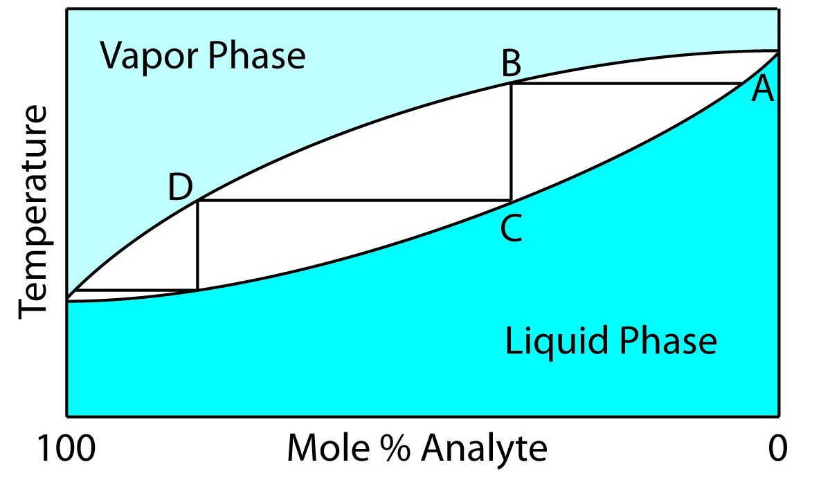
Figure 7.17: Boiling point versus composition diagram for a near-ideal solution consisting of a low-boiling analyte and a high-boiling interferent. The horizontal lines represent vaporization equilibria and the vertical lines represent condensation equilibria. See the text for additional details.
Two experimental set-ups for distillations are shown in Figure 7.18. The simple distillation apparatus shown in Figure 7.18a does not produce a very efficient separation, and is useful only for separating a volatile analyte (or interferent) from a non-volatile interferent (or analyte), or for an analyte and interferent whose boiling points differ by more than 150oC. A more efficient separation is achieved by a fractional distillation (Figure 7.18b). Packing the distillation column with a high surface area material, such as a steel sponge or glass beads, provides more opportunity for the repeated process of vaporization and condensation necessary to effect a complete separation.
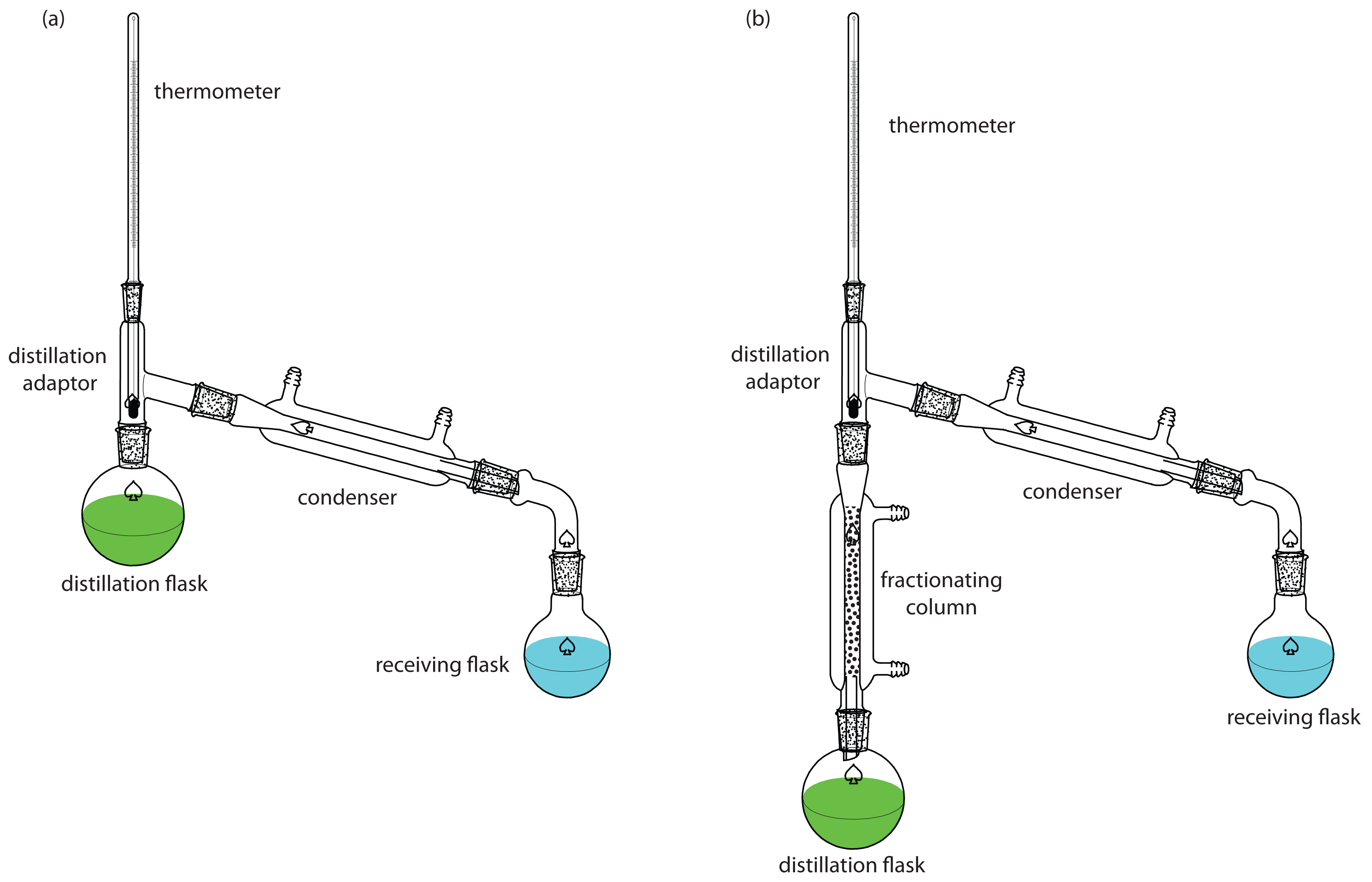
Figure 7.18: Typical experimental set-up for (a) a simple distillation, and (b) a fractional distillation.
When the sample is a solid, sublimation may provide a useful separation of the analyte and the interferent. The sample is heated at a temperature and pressure below the analyte’s triple point, allowing it to vaporize without passing through the liquid state. Condensing the vapor recovers the purified analyte (Figure 7.19). A useful analytical example of sublimation is the isolation of amino acids from fossil mollusk shells and deep-sea sediments.13
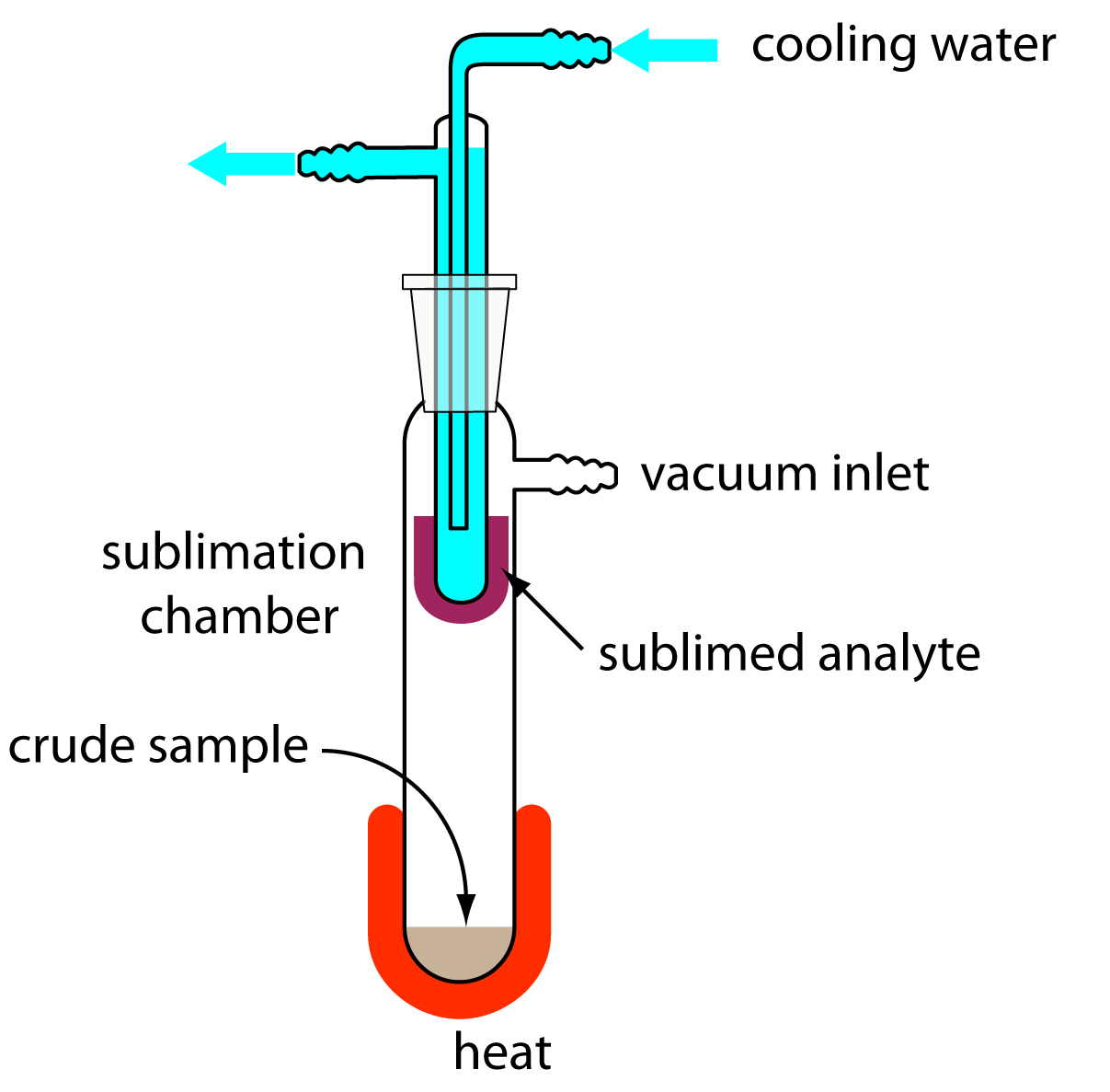
Figure 7.19: Typical experimental setup for a sublimation. The sample is placed in the sublimation chamber, which may be evacuated. Heating the sample causes the analyte to vaporize and sublime onto a cooled probe. Modified from Slashme (commons.wikipedia.org).
Recrystallization is another method for purifying a solid. A solvent is chosen in which the analyte’s solubility is significant when the solvent is hot, and minimal when the solvent is cold. The interferents must be less soluble in the hot solvent than the analyte, or present in much smaller amounts. After heating a portion of the solvent in an Erlenmeyer flask, small amounts of the sample are added until undissolved sample is visible. Additional hot solvent is added until the sample redissolves, or until only insoluble impurities remain. This process of adding sample and solvent is repeated until the entire sample has been added to the Erlenmeyer flask. Any insoluble impurities are removed by filtering the hot solution. The solution is allowed to cool slowly, promoting the growth of large, pure crystals, and then cooled in an ice bath to minimize solubility losses. The purified sample is isolated by filtration and rinsed to remove any soluble impurities. Finally, the sample is dried to remove any remaining traces of the solvent. Further purification, if necessary, can be accomplished by additional recrystallizations.
Changes in Chemical State
Distillation, sublimation, and recrystallization use a change in physical state as a means of separation. Chemical reactivity also can be a useful tool for separating analytes and interferents. For example, we can separate SiO2 from a sample by reacting it with HF to form SiF4. Because SiF4 is volatile, it is easy to remove by evaporation. If we wish to collect the reaction’s volatile product, then a distillation is possible. For example, we can isolate the NH4+ in a sample by making the solution basic and converting it to NH3. The ammonia is then removed by distillation. Table 7.7 provides additional examples of this approach for isolating inorganic ions.
| Analyte | Treatment | Isolated Species |
|---|---|---|
| CO32− | CO32−(aq)+ 2H3O+(aq) → CO2(g) + 3H2O(l) | CO2 |
| NH4+ | NH4+(aq) + OH−(aq) → NH3(g) + H2O(l) | NH3 |
| SO32− | SO32−(aq) + 2H3O+(aq) → SO2(g) + 3H2O(l) | SO2 |
| S2− | S2−(aq) + 2H3O+(aq) → H2S(g) + 2H2O(l) | H2S |
Another reaction for separating analytes and interferents is precipitation. Two important examples of using a precipitation reaction in a separation are the pH-dependent solubility of metal oxides and hydroxides, and the solubility of metal sulfides.
Separations based on the pH-dependent solubility of oxides and hydroxides usually use strong acids, strong bases, or an NH3/NH4Cl buffer. Most metal oxides and hydroxides are soluble in hot concentrated HNO3, although a few oxides, such as WO3, SiO2, and SnO2 remain insoluble even under these harsh conditions. In determining the amount of Cu in brass, for example, we can avoid an interference from Sn by dissolving the sample with a strong acid and filtering to remove the solid residue of SnO2.
Most metals form a hydroxide precipitate in the presence of concentrated NaOH. Those metals forming amphoteric hydroxides, however, do not precipitate because they react to form higher-order hydroxo-complexes. For example, Zn2+ and Al3+ do not precipitate in concentrated NaOH because the form the soluble complexes Zn(OH)3– and Al(OH)4–. The solubility of Al3+ in concentrated NaOH allows us to isolate aluminum from impure samples of bauxite, an ore of Al2O3. After crushing the ore, we place it in a solution of concentrated NaOH, dissolving the Al2O3 and forming Al(OH)4–. Other oxides in the ore, such as Fe2O3 and SiO2, remain insoluble. After filtering, we recover the aluminum as a precipitate of Al(OH)3 by neutralizing some of the OH– with acid.
The pH of an NH3/NH4Cl buffer (pKa = 9.26) is sufficient to precipitate most metals as the hydroxide. The alkaline earths and alkaline metals, however, do not precipitate at this pH. In addition, metal ions that form soluble complexes with NH3, such as Cu2+, Zn2+, Ni2+, and Co2+ also do not precipitate under these conditions.
The use of S2– as a precipitating reagent is one of the earliest examples of a separation technique. In Fresenius’s 1881 text A System of Instruction in Quantitative Chemical Analysis, sulfide is frequently used to separate metal ions from the remainder of the sample’s matrix.14 Sulfide is a useful reagent for separating metal ions for two reasons: (1) most metal ions, except for the alkaline earths and alkaline metals, form insoluble sulfides; and (2) these metal sulfides show a substantial variation in solubility. Because the concentration of S2– is pH-dependent, we can control which metal precipitates by adjusting the pH. For example, in Fresenius’s gravimetric procedure for determining Ni in ore samples (see Figure 1.1 in Chapter 1 for a schematic diagram of this procedure), sulfide is used three times as a means of separating Co2+ and Ni2+ from Cu2+ and, to a lesser extent, from Pb2+.
7.6.5 Separations Based on a Partitioning Between Phases
The most important group of separation techniques uses a selective partitioning of the analyte or interferent between two immiscible phases. If we bring a phase containing a solute, S, into contact with a second phase, the solute partitions itself between the two phases, as shown by the following equilibrium reaction.
\[\textrm S_\textrm{phase 1}\rightleftharpoons \textrm S_\textrm{phase 2}\tag{7.20}\]
The equilibrium constant for reaction 7.20
\[K_\textrm D=\mathrm{\dfrac{[S_{phase\;2}]}{[S_{phase\;1}]}}\]
is called the distribution constant or partition coefficient. If KD is sufficiently large, then the solute moves from phase 1 to phase 2. The solute remains in phase 1 if the partition coefficient is sufficiently small. When we bring a phase containing two solutes into contact with a second phase, if KD is favorable for only one of the solutes a separation of the solutes is possible. The physical states of the phases are identified when describing the separation process, with the phase containing the sample listed first. For example, if the sample is in a liquid phase and the second phase is a solid, then the separation involves liquid–solid partitioning.
Extraction Between Two Phases
We call the process of moving a species from one phase to another phase an extraction. Simple extractions are particularly useful for separations where only one component has a favorable partition coefficient. Several important separation techniques are based on a simple extraction, including liquid–liquid, liquid–solid, solid–liquid, and gas–solid extractions.
Liquid–Liquid Extractions
A liquid–liquid extraction is usually accomplished with a separatory funnel (Figure 7.20). After placing the two liquids in the separatory funnel, we shake the funnel to increase the surface area between the phases. When the extraction is complete, we allow the liquids to separate. The stopcock at the bottom of the separatory funnel allows us to remove the two phases.

Figure 7.20: Example of a liquid–liquid extraction using a separatory funnel. (a) Before the extraction, 100% of the analyte is in phase 1. (b) After the extraction, most of the analyte is in phase 2, although some analyte remains in phase 1. Although one liquid–liquid extraction can result in the complete transfer of analyte, a single extraction usually is not sufficient. See Section 7G for a discussion of extraction efficiency and multiple extractions.
We also can carry out a liquid–liquid extraction without a separatory funnel by adding the extracting solvent to the sample container. Pesticides in water, for example, are preserved in the field by extracting them into a small volume of hexane. Liquid–liquid microextractions, in which the extracting phase is a 1-mL drop suspended from a microsyringe (Figure 7.21), also have been described.15 Because of its importance, a more thorough discussion of liquid–liquid extraction is in section 7G.

Figure 7.21: Schematic of a liquid–liquid microextraction showing a syringe needle with a μL drop of the extracting solvent.
Solid Phase Extractions
In a solid phase extraction of a liquid sample, we pass the sample through a cartridge containing a solid adsorbent, several examples of which are shown in Figure 7.22. The choice of adsorbent is determined by the species we wish to separate. Table 7.8 provides several representative examples of solid adsorbents and their applications.

Figure 7.22 Selection of solid phase extraction cartridges for liquid samples. The solid adsorbent is the white material in each cartridge. Source: Jeff Dahl (commons.wikipedia.org).
| Adsorbent | Structure | Properties and Uses |
|---|---|---|
| silica | 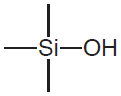 |
|
| aminopropyl | 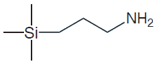 |
|
| cyanopropyl |  |
|
| diol |  |
|
| octadecyl (C-18) | —C18H37 |
|
| octyl (C-8) | —C8H17 |
|
As an example, let’s examine a procedure for isolating the sedatives secobarbital and phenobarbital from serum samples using a C-18 solid adsorbent.16 Before adding the sample, the solid phase cartridge is rinsed with 6 mL each of methanol and water. Next, a 500-μL sample of serum is pulled through the cartridge, with the sedatives and matrix interferents retained by a liquid–solid extraction (Figure 7.23a). Washing the cartridge with distilled water removes any interferents (Figure 7.23b). Finally, we elute the sedatives using 500 μL of acetone (Figure 7.23c). In comparison to a liquid–liquid extraction, a solid phase extraction has the advantage of being easier, faster, and requiring less solvent.

Figure 7.23 Steps in a typical solid phase extraction. After preconditioning the solid phase cartridge with solvent, (a) the sample is added to the cartridge, (b) the sample is washed to remove interferents, and (c) the analytes eluted.
Continuous Extractions
An extraction is possible even if the analyte has an unfavorable partition coefficient, provided that the sample’s other components have significantly smaller partition coefficients. Because the analyte’s partition coefficient is unfavorable, a single extraction will not recover all the analyte. Instead we continuously pass the extracting phase through the sample until a quantitative extraction is achieved.
A continuous extraction of a solid sample is carried out using a Soxhlet extractor (Figure 7.24). The extracting solvent is placed in the lower reservoir and heated to its boiling point. Solvent in the vapor phase moves upwards through the tube on the far right side of the apparatus, reaching the condenser where it condenses back to the liquid state. The solvent then passes through the sample, which is held in a porous cellulose filter thimble, collecting in the upper reservoir. When the solvent in the upper reservoir reaches the return tube’s upper bend, the solvent and extracted analyte are siphoned back to the lower reservoir. Over time the analyte’s concentration in the lower reservoir increases.
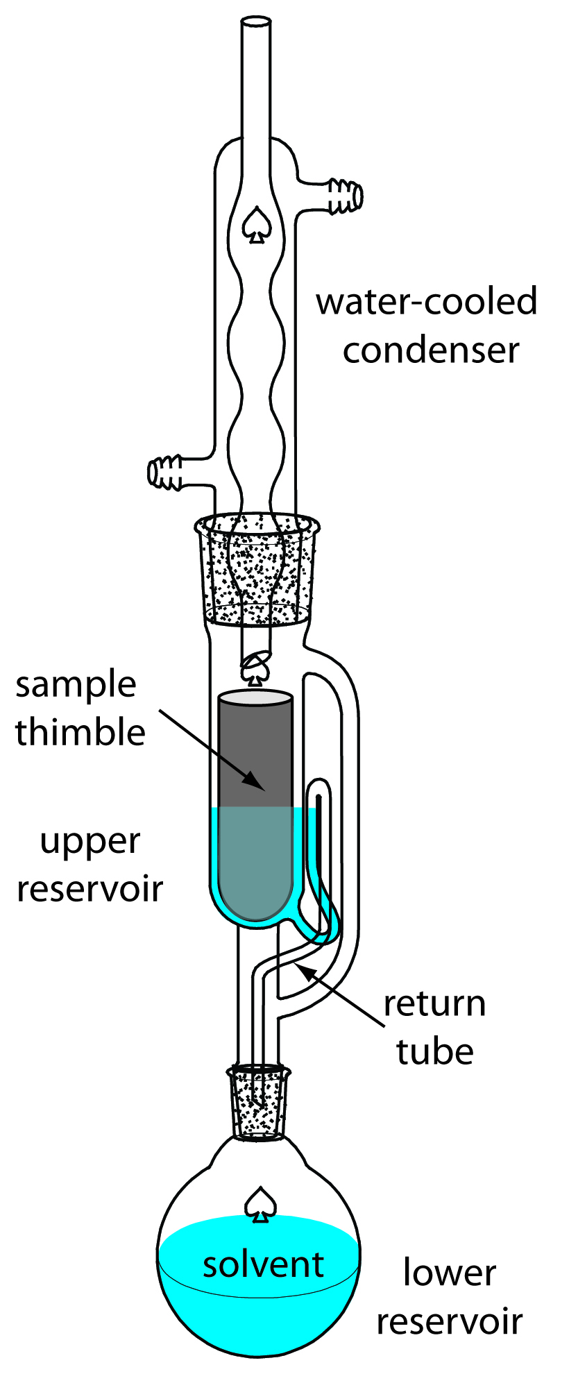
Figure 7.24 Soxhlet extractor. See text for details.
Microwave-assisted extractions have replaced Soxhlet extractions in some applications.17 The process is the same as that described earlier for a microwave digestion. After placing the sample and the solvent in a sealed digestion vessel, a microwave oven is used to heat the mixture. Using a sealed digestion vessel allows the extraction to take place at a higher temperature and pressure, reducing the amount of time needed for a quantitative extraction. In a Soxhlet extraction the temperature is limited by the solvent’s boiling point at atmospheric pressure. When acetone is the solvent, for example, a Soxhlet extraction is limited to 56oC, but a microwave extraction can reach 150oC.
Two other continuous extractions deserve mention. Volatile organic compounds (VOCs) can be quantitatively removed from liquid samples by a liquid–gas extraction. As shown in Figure 7.25, an inert purging gas, such as He, is passed through the sample. The purge gas removes the VOCs, which are swept to a primary trap where they collect on a solid absorbent. A second trap provides a means for checking to see if the primary trap’s capacity is exceeded. When the extraction is complete, the VOCs are removed from the primary trap by rapidly heating the tube while flushing with He. This technique is known as a purge-and-trap. Because the analyte’s recovery may not be reproducible, an internal standard is necessary for quantitative work.
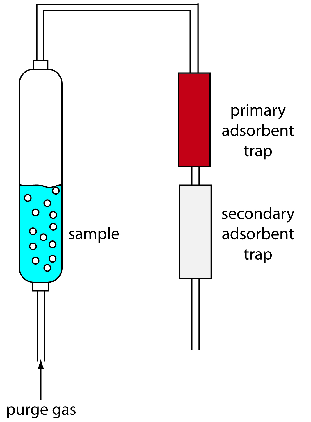
Figure 7.25 Schematic diagram of a purge-and-trap system for extracting volatile analytes. The purge gas releases the analytes, which subsequently collect in the primary adsorbent trap. The secondary adsorption trap is monitored for evidence of the analyte’s breakthrough.
Continuous extractions also can be accomplished using supercritical fluids.18 If we heat a substance above its critical temperature and pressure, it forms a supercritical fluid whose properties are between those of a gas and a liquid. A supercritical fluid is a better solvent than a gas, which makes it a better reagent for extractions. In addition, a supercritical fluid’s viscosity is significantly less than that of a liquid, making it easier to push it through a particulate sample. One example of a supercritical fluid extraction is the determination of total petroleum hydrocarbons (TPHs) in soils, sediments, and sludges using supercritical CO2.19 An approximately 3-g sample is placed in a 10-mL stainless steel cartridge and supercritical CO2 at a pressure of 340 atm and a temperature of 80oC is passed through the cartridge for 30 minutes at flow rate of 1–2 mL/min. To collect the TPHs, the effluent from the cartridge is passed through 3 mL of tetrachloroethylene at room temperature. At this temperature the CO2 reverts to the gas phase and is released to the atmosphere.
Chromatographic Separations
In an extraction, the sample is one phase and we extract the analyte or the interferent into a second phase. We also can separate the analyte and interferents by continuously passing one sample-free phase, called the mobile phase, over a second sample-free phase that remains fixed or stationary. The sample is injected into the mobile phase and the sample’s components partition themselves between the mobile phase and the stationary phase. Those components with larger partition coefficients are more likely to move into the stationary phase, taking a longer time to pass through the system. This is the basis of all chromatographic separations. Chromatography provides both a separation of analytes and interferents, and a means for performing a qualitative or quantitative analysis for the analyte. For this reason a more thorough treatment of chromatography is found in Chapter 12.