6.6: Ladder Diagrams

When developing or evaluating an analytical method, we often need to understand how the chemistry taking place affects our results. Suppose we wish to isolate Ag⁺ by precipitating it as AgCl. If we also a need to control pH, then we must use a reagent that will not adversely affects the solubility of AgCl. It is a mistake to add NH₃ to the reaction mixture, for example, because it increases the solubility of AgCl (reaction 6.29). One of the primary sources of determinate errors in many analytical methods is failing to account for potential chemical interferences.

In this section we introduce the ladder diagram as a simple graphical tool for evaluating the equilibrium chemistry.² Using ladder diagrams we will be able to determine what reactions occur when combining several reagents, estimate the approximate composition of a system at equilibrium, and evaluate how a change to solution conditions might affect an analytical method.

Note

Ladder diagrams are a great tool for helping you to think intuitively about analytical chemistry. We will make frequent use of them in the chapters to follow.

6.6.1 Ladder Diagrams for Acid–Base Equilibria

Let’s use acetic acid, CH₃COOH, to illustrate the process of drawing and interpreting an acid–base ladder diagram. Before drawing the diagram, however, let’s consider the equilibrium reaction in more detail. The equilibrium constant expression for acetic acid’s dissociation reaction

\[\mathrm{CH_3COOH}(aq)+\mathrm{H_2O}(l)\rightleftharpoons\mathrm{H_3O^+}(aq)+\mathrm{CH_3COO^-}(aq)\]

is

\[K_\textrm a=\mathrm{\dfrac{[CH_3COO^-][H_3O^+]}{[CH_3COOH]}}=1.75\times10^{-5}\]

Taking the logarithm of each term in this equation, and multiplying through by –1 gives

\[-\log K_\mathrm a=-\log\mathrm{[H_3O^+]-\log\dfrac{[CH_3COO^-]}{[CH_3COOH]}=4.76}\]

Replacing the negative log terms with p-functions and rearranging the equation, leaves us with the result shown here.

\[\textrm{pH}=\textrm pK_\textrm a+\log\mathrm{\dfrac{[CH_3COO^-]}{[CH_3COOH]}}=4.76\tag{6.31}\]

Equation 6.31 tells us a great deal about the relationship between pH and the relative amounts of acetic acid and acetate at equilibrium. If the concentrations of CH₃COOH and CH₃COO^– are equal, then equation 6.31 reduces to

\[\textrm{pH}=\textrm pK_\textrm a+\log(1)=\textrm pK_\textrm a=4.76\]

If the concentration of CH₃COO^– is greater than that of CH₃COOH, then the log term in equation 6.31 is positive and

\[\mathrm{pH>p}K_\mathrm a\hspace{3mm}or\hspace{3mm}\mathrm{pH}>4.76\]

This is a reasonable result because we expect the concentration of the conjugate base, CH₃COO^–, to increase as the pH increases. Similar reasoning shows that the concentration of CH₃COOH exceeds that of CH₃COO^– when

\[\mathrm{pH<p}K_\mathrm a\hspace{3mm}or\hspace{3mm}\mathrm{pH}<4.76\]

Now we are ready to construct acetic acid’s ladder diagram (Figure 6.3). First, we draw a vertical arrow representing the solution’s pH, with smaller (more acidic) pH levels at the bottom and larger (more basic) pH levels at the top. Second, we draw a horizontal line at a pH equal to acetic acid’s pK_a value. This line, or step on the ladder, divides the pH axis into regions where either CH₃COOH or CH₃COO^– is the predominate species. This completes the ladder diagram.

Using the ladder diagram, it is easy to identify the predominate form of acetic acid at any pH. At a pH of 3.5, for example, acetic acid exists primarily as CH₃COOH. If we add sufficient base to the solution such that the pH increases to 6.5, the predominate form of acetic acid is CH₃COO^–.

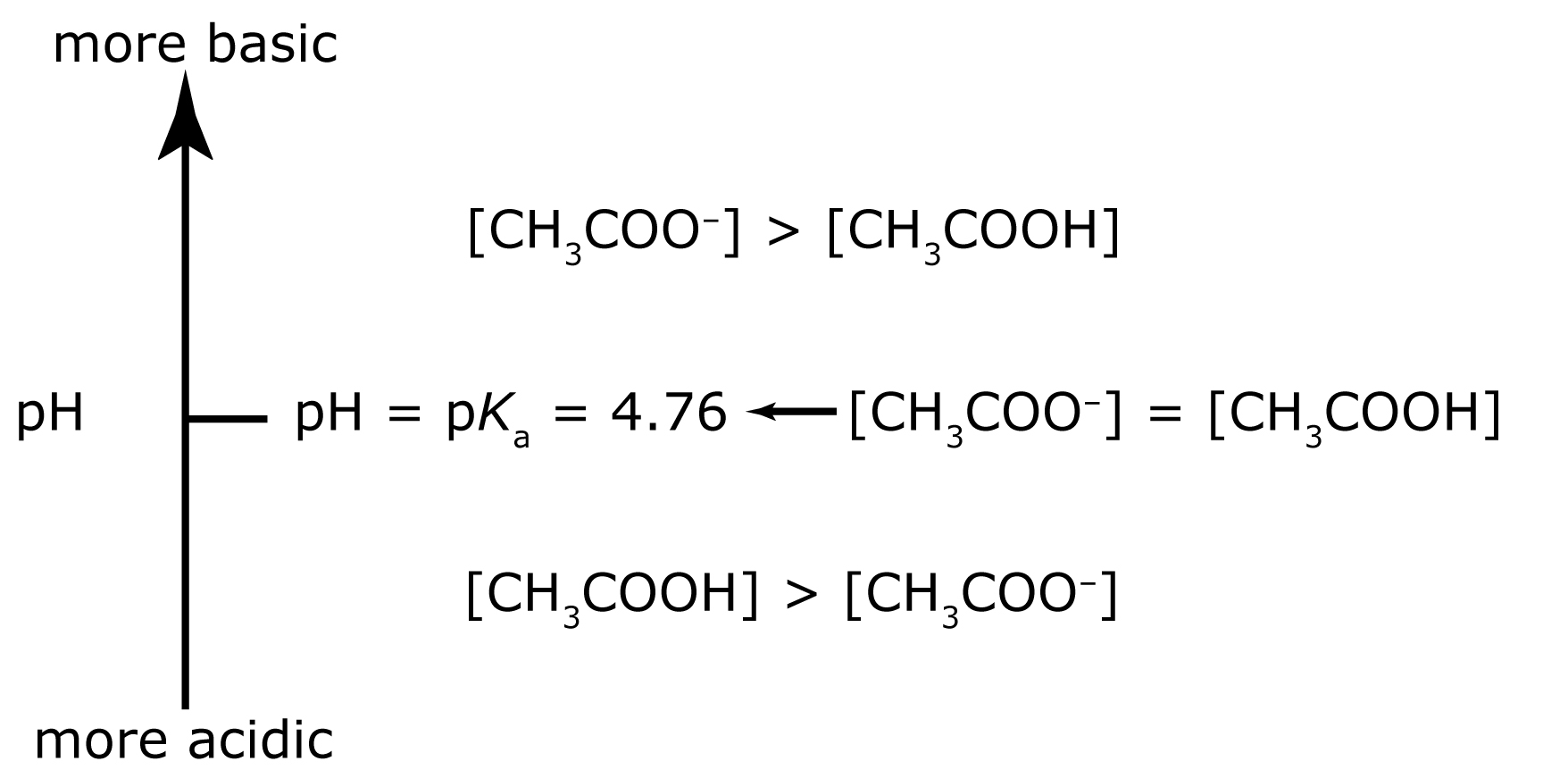
Figure 6.3 Acid–base ladder diagram for acetic acid showing the relative concentrations of CH₃COOH and CH₃COO^–. A simpler version of this ladder diagram dispenses with the equalities and shows only the predominate species in each region.

Example 6.7

Draw a ladder diagram for the weak base p-nitrophenolate and identify its predominate form at a pH of 6.00.

Solution

To draw a ladder diagram for a weak base, we simply draw the ladder diagram for its conjugate weak acid. From Appendix 12, the pK_a for p-nitrophenol is 7.15. The resulting ladder diagram is shown in Figure 6.4. At a pH of 6.00, p-nitrophenolate is present primarily in its weak acid form.

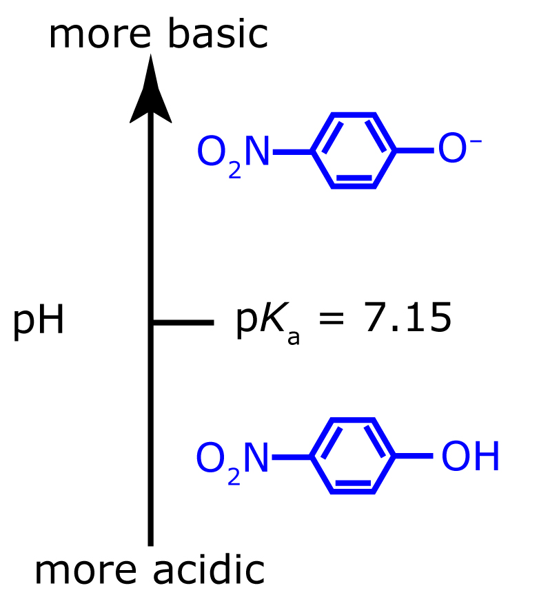
Figure 6.4 Acid–base ladder diagram for p-nitrophenolate.

Exercise 6.5

Draw a ladder diagram for carbonic acid, H₂CO₃. Because H₂CO₃ is a diprotic weak acid, your ladder diagram will have two steps. What is the predominate form of carbonic acid when the pH is 7.00? Relevant equilibrium constants are in Appendix 11.

Click here to review your answer to this exercise.

Ladder diagrams are particularly useful for evaluating the reactivity between a weak acid and a weak base. Figure 6.5 shows a single ladder diagram for acetic acid/acetate and p-nitrophenol/p-nitrophenolate. An acid and a base can not co-exist if their respective areas of predominance do not overlap. If we mix together solutions of acetic acid and sodium p-nitrophenolate, the reaction

6.32

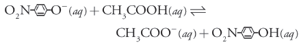
occurs because the areas of predominance for acetic acid and p-nitrophenolate do not overlap. The solution’s final composition depends on which species is the limiting reagent. The following example shows how we can use the ladder diagram in Figure 6.5 to evaluate the result of mixing together solutions of acetic acid and p-nitrophenolate.

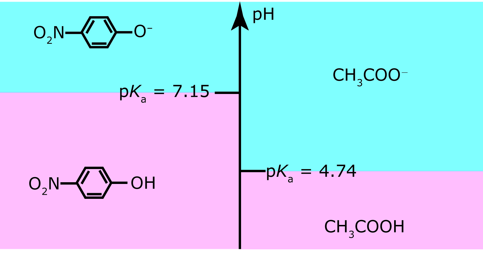
Figure 6.5 Acid–base ladder diagram showing the areas of predominance for acetic acid/acetate and forp-nitrophenol/p-nitrophenolate. The areas in blue shading show the pH range where the weak bases are the predominate species; the weak acid forms are the predominate species in the areas shown in pink shading.

Example 6.8

Predict the approximate pH and the final composition of mixing together 0.090 moles of acetic acid and 0.040 moles of p-nitrophenolate.

Solution

The ladder diagram in Figure 6.5 indicates that the reaction between acetic acid and p-nitrophenolate is favorable. Because acetic acid is in excess, we assume that the reaction of p-nitrophenolate to p-nitrophenol is complete. At equilibrium essentially no p-nitrophenolate remains and there are 0.040 mol of p-nitrophenol. Converting p-nitrophenolate to p-nitrophenol consumes 0.040 moles of acetic acid; thus

\[\mathrm{moles\;CH_3COOH=0.090-0.040=0.050\;mol}\]

\[\mathrm{moles\;CH_3COO^-=0.040\;mol}\]

According to the ladder diagram, the pH is 4.76 when there are equal amounts of CH₃COOH and CH₃COO^–. Because we have slightly more CH₃COOH than CH₃COO^–, the pH is slightly less than 4.76.

Exercise 6.6

Using Figure 6.5, predict the approximate pH and the composition of a solution formed by mixing together 0.090 moles of p-nitrophenolate and 0.040 moles of acetic acid.

Click here to review your answer to this exercise.

If the areas of predominance for an acid and a base overlap, then practically no reaction occurs. For example, if we mix together solutions of CH₃COO^– and p-nitrophenol, there is no significant change in the moles of either reagent. Furthermore, the pH of the mixture must be between 4.76 and 7.15, with the exact pH depending upon the relative amounts of CH₃COO^– and p-nitrophenol.

We also can use an acid–base ladder diagram to evaluate the effect of pH on other equilibria. For example, the solubility of CaF₂

\[\mathrm{CaF_2}(s)\rightleftharpoons\mathrm{Ca^{2+}}(aq)+\mathrm{2F^-}(aq)\]

is affected by pH because F^– is a weak base. Using Le Châtelier’s principle, converting F^– to HF increases the solubility of CaF₂. To minimize the solubility of CaF₂ we need to maintain the solution’s pH so that F^– is the predominate species. The ladder diagram for HF (Figure 6.6) shows us that maintaining a pH of more than 3.17 minimizes solubility losses.

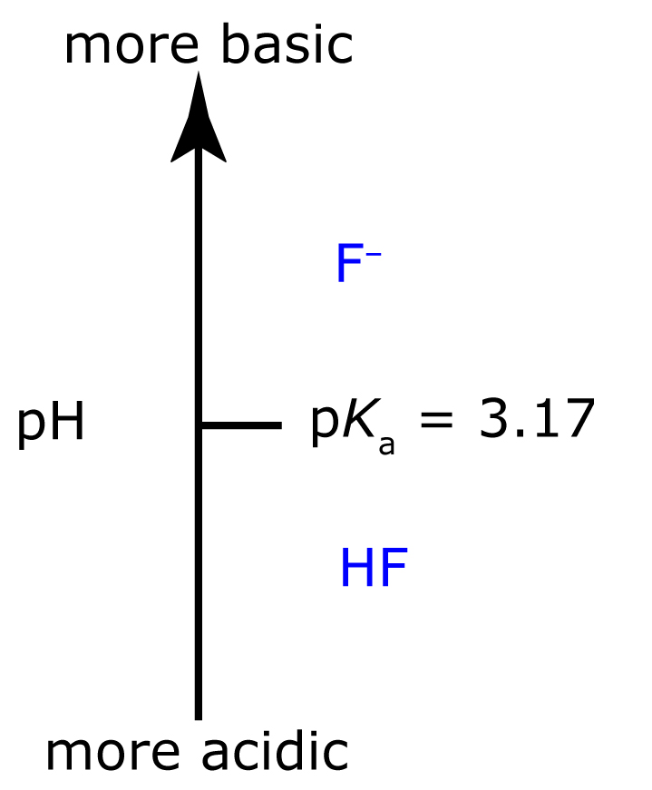
Figure 6.6 Acid–base ladder diagram for HF. To minimize the solubility of CaF₂, we need to keep the pH above 3.17, with more basic pH levels leading to smaller solubility losses. See Chapter 8 for a more detailed discussion.

6.6.2 Ladder Diagrams for Complexation Equilibria

We can apply the same principles for constructing and interpreting acid–base ladder diagrams to equilibria involving metal–ligand complexes. For a complexation reaction we define the ladder diagram’s scale using the concentration of uncomplexed, or free ligand, pL. Using the formation of Cd(NH₃)²⁺ as an example

\[\mathrm{Cd^{2+}}(aq)+\mathrm{NH_3}(aq)\rightleftharpoons\mathrm{Cd(NH_3)^{2+}}(aq)\]

we can easily show that logK₁ is the dividing line between the areas of predominance for Cd²⁺ and Cd(NH₃)²⁺.

\[K_1=\mathrm{\dfrac{[Cd(NH_3)^{2+}]}{[Cd^{2+}][NH_3]}=3.55\times10^2}\]

\[\log K_1=\log\mathrm{\dfrac{[Cd(NH_3)^{2+}]}{[Cd^{2+}]}}-\log[\mathrm{NH_3}]=2.55\]

\[\log K_1=\log\mathrm{\dfrac{[Cd(NH_3)^{2+}]}{[Cd^{2+}]}+pNH_3}=2.55\]

\[\mathrm{pNH_3}{}=\log K_1+\log\mathrm{\dfrac{[Cd^{2+}]}{[Cd(NH_3)^{2+}]}}=2.55\]

Thus, Cd²⁺ is the predominate species when pNH₃ is greater than 2.55 (a concentration of NH₃ smaller than 2.82 × 10^–3 M) and for pNH₃ values less than 2.55, Cd(NH₃)²⁺ is the predominate species. Figure 6.7 shows a complete metal–ligand ladder diagram for Cd²⁺ and NH₃.

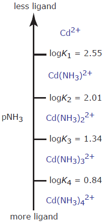
Figure 6.7 Metal–ligand ladder diagram for Cd²⁺–NH₃ complexation reactions. Note that higher-order complexes form when pNH₃ is smaller (which corresponds to larger concentrations of NH₃).

Example 6.9

Draw a single ladder diagram for the Ca(EDTA)^2– and Mg(EDTA)^2– metal–ligand complexes. Using your ladder diagram, predict the result of adding 0.080 moles of Ca²⁺ to 0.060 moles of Mg(EDTA)^2–. EDTA is an abbreviation for the ligand ethylenediaminetetraacetic acid.

Solution

Figure 6.8 shows the ladder diagram for this system of metal–ligand complexes. Because the predominance regions for Ca²⁺ and Mg(EDTA)^2- do not overlap, the reaction

\[\mathrm{Ca^{2+}}(aq)+\mathrm{Mg(EDTA)^{2-}}(aq)\rightleftharpoons\mathrm{Ca(EDTA)^{2-}}(aq)+\mathrm{Mg^{2+}}(aq)\]

takes place. Because Ca²⁺ is the excess reagent, the composition of the final solution is approximately

\[\mathrm{moles\;Ca^{2+}=0.080-0.060=0.020\;mol}\]

\[\mathrm{moles\;Ca(EDTA)^{2-}=0.060\;mol}\]

\[\mathrm{moles\;Mg^{2+}=0.060\;mol}\]

\[\mathrm{moles\;Mg(EDTA)^{2-}=0\;mol}\]

Figure 6.8 Metal–ligand ladder diagram for Ca(EDTA)^2– and for Mg(EDTA)^2–. The areas with blue shading shows the pEDTA range where the free metal ions are the predominate species; the metal–ligand complexes are the predominate species in the areas shown with pink shading.

The metal–ligand ladder diagram in Figure 6.7 uses stepwise formation constants. We can also construct ladder diagrams using cumulative formation constants. The first three stepwise formation constants for the reaction of Zn²⁺ with NH₃

\[\mathrm{Zn^{2+}}(aq)+\mathrm{NH_3}(aq)\rightleftharpoons\mathrm{Zn(NH_3)^{2+}}(aq)\hspace{5mm}K_1=1.6\times10^2\]

\[\mathrm{Zn(NH_3)^{2+}}(aq)+\mathrm{NH_3}(aq)\rightleftharpoons\mathrm{Zn(NH_3)_2^{2+}}(aq)\hspace{5mm}K_2=1.95\times10^2\]

\[\mathrm{Zn(NH_3)_2^{2+}}(aq)+\mathrm{NH_3}(aq)\rightleftharpoons\mathrm{Zn(NH_3)_3^{2+}}(aq)\hspace{5mm}K_3=2.3\times10^2\]

show that the formation of Zn(NH₃)₃²⁺ is more favorable than the formation of Zn(NH₃)²⁺ or Zn(NH₃)₂²⁺. For this reason, the equilibrium is best represented by the cumulative formation reaction shown here.

\[\mathrm{Zn^{2+}}(aq)+\mathrm{3NH_3}(aq)\rightleftharpoons\mathrm{Zn(NH_3)_3^{2+}}(aq)\hspace{5mm}\beta_3=7.2\times10^6\]

Note

Because K₃ is greater than K₂, which is greater than K₁, the formation of the metal-ligand complex Zn(NH₃)₃²⁺ is more favorable than the formation of the other metal ligand complexes. For this reason, at lower values of pNH₃ the concentration of Zn(NH₃)₃²⁺ is larger than that for Zn(NH₃)₂²⁺ and Zn(NH₃)²⁺. The value of β₃ is

\[\beta_3=K_1\times K_2\times K_3\]

To see how we incorporate this cumulative formation constant into a ladder diagram, we begin with the reaction’s equilibrium constant expression.

\[\mathrm{\beta_3=\dfrac{[Zn(NH_3)_3^{2+}]}{[Zn^{2+}][NH_3]^3}}\]

Taking the log of each side gives

\[\mathrm{\log\beta_3=\log\dfrac{[Zn(NH_3)_3^{2+}]}{[Zn^{2+}]}-3\log[NH_3]}\]

or

\[\mathrm{pNH_3=\dfrac{1}{3}\log\beta_3+\dfrac{1}{3}\log\dfrac{[Zn]}{[Zn(NH_3)_3^{2+}]}}\]

When the concentrations of Zn²⁺ and Zn(NH₃)₃²⁺ are equal, then

\[\mathrm{pNH_3=\dfrac{1}{3}\log\beta_3=2.29}\]

In general, for the metal–ligand complex ML_n, the step for a cumulative formation constant is

\[\mathrm{pL}=\dfrac{1}{n}\log\beta_n\]

Figure 6.9 shows the complete ladder diagram for the Zn²⁺–NH₃ system.

Figure 6.9 Ladder diagram for Zn²⁺–NH₃ metal–ligand complexation reactions showing both a step based on a cumulative formation constant, and a step based on a stepwise formation constant.

6.6.3 Ladder Diagram for Oxidation/Reduction Equilibria

We also can construct ladder diagrams to help evaluate redox equilibria. Figure 6.10 shows a typical ladder diagram for two half-reactions in which the scale is the potential, E. The Nernst equation defines the areas of predominance. Using the Fe³⁺/Fe²⁺ half-reaction as an example, we write

\[E=E^\circ-\dfrac{RT}{nF}\ln\mathrm{\dfrac{[Fe^{2+}]}{[Fe^{3+}]}}=+0.771-0.05916\log\mathrm{\dfrac{[Fe^{2+}]}{[Fe^{3+}]}}\]

At potentials more positive than the standard state potential, the predominate species is Fe³⁺, whereas Fe²⁺ predominates at potentials more negative than E^o. When coupled with the step for the Sn⁴⁺/Sn²⁺ half-reaction we see that Sn²⁺ is a useful reducing agent for Fe³⁺. If Sn²⁺ is in excess, the potential of the resulting solution is near +0.151 V.

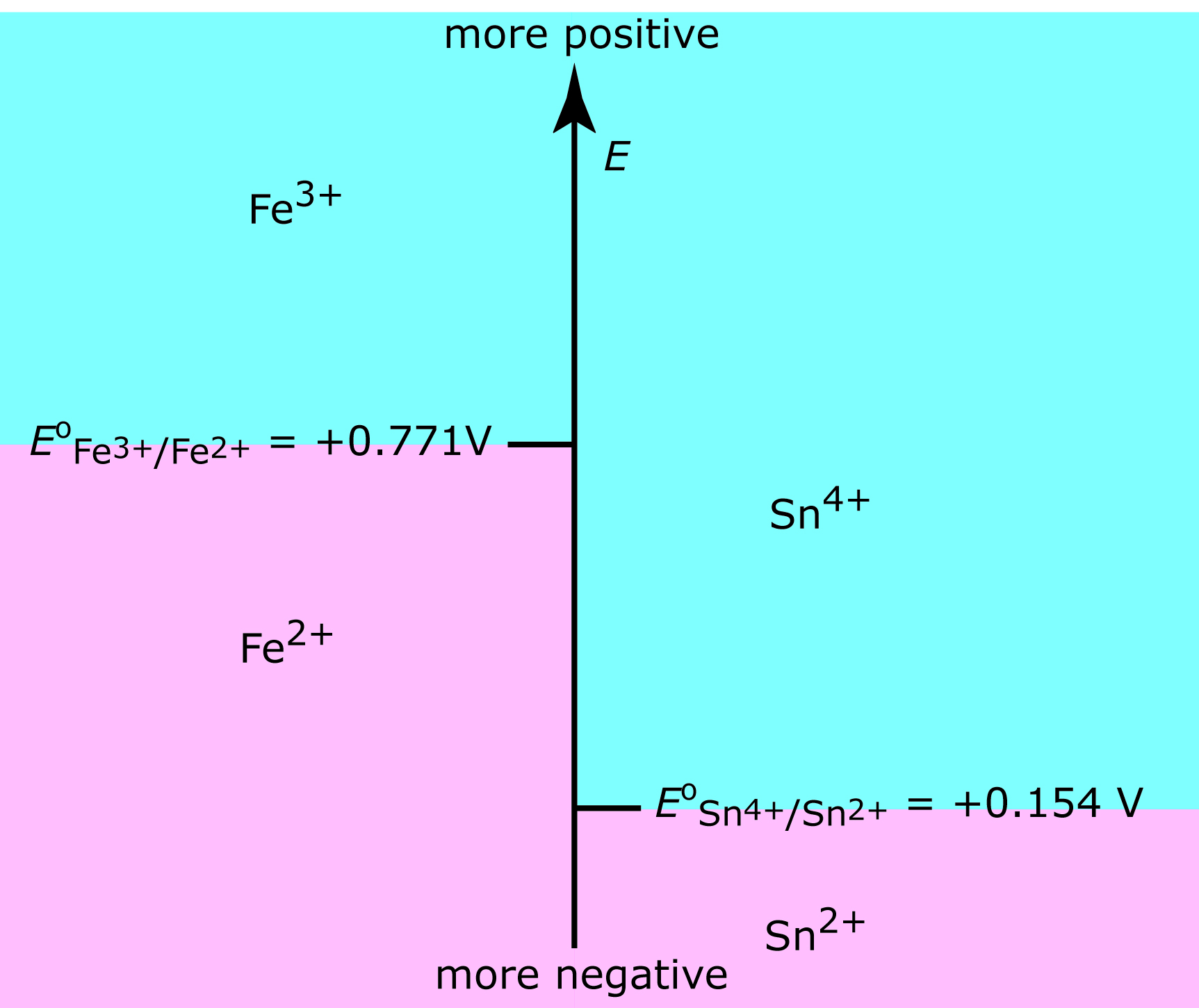
Figure 6.10 Redox ladder diagram for Fe³⁺/Fe²⁺ and for Sn⁴⁺/Sn²⁺. The areas with blue shading show the potential range where the oxidized forms are the predominate species; the reduced forms are the predominate species in the areas shown with pink shading. Note that a more positive potential favors the oxidized form.

Because the steps on a redox ladder diagram are standard state potentials, complications arise if solutes other than the oxidizing agent and reducing agent are present at non-standard state concentrations. For example, the potential for the half-reaction

\[\mathrm{UO_2^{2+}}(aq)+\mathrm{4H_3O^+}(aq)+2e^-\rightleftharpoons\mathrm{U^{4+}}(aq)+\mathrm{6H_2O}(l)\]

depends on the solution’s pH. To define areas of predominance in this case we begin with the Nernst equation

\[E=+0.327-\dfrac{0.05916}{2}\log\mathrm{\dfrac{[U^{4+}]}{[UO_2^{2+}][H_3O^+]^4}}\]

and factor out the concentration of H₃O⁺.

\[E=\mathrm{+0.327+\dfrac{0.05916}{2}\log[H_3O^+]^4-\dfrac{0.05916}{2}\log\dfrac{[U^{4+}]}{[UO_2^{2+}]}}\]

From this equation we see that the area of predominance for UO₂²⁺ and U⁴⁺ is defined by a step whose potential is

\[E=\mathrm{+0.327+\dfrac{0.05916}{2}\log[H_3O^+]^4=+0.327-0.1183pH}\]

Figure 6.11 shows how pH affects the step for the UO₂²⁺/U⁴⁺ half-reaction.

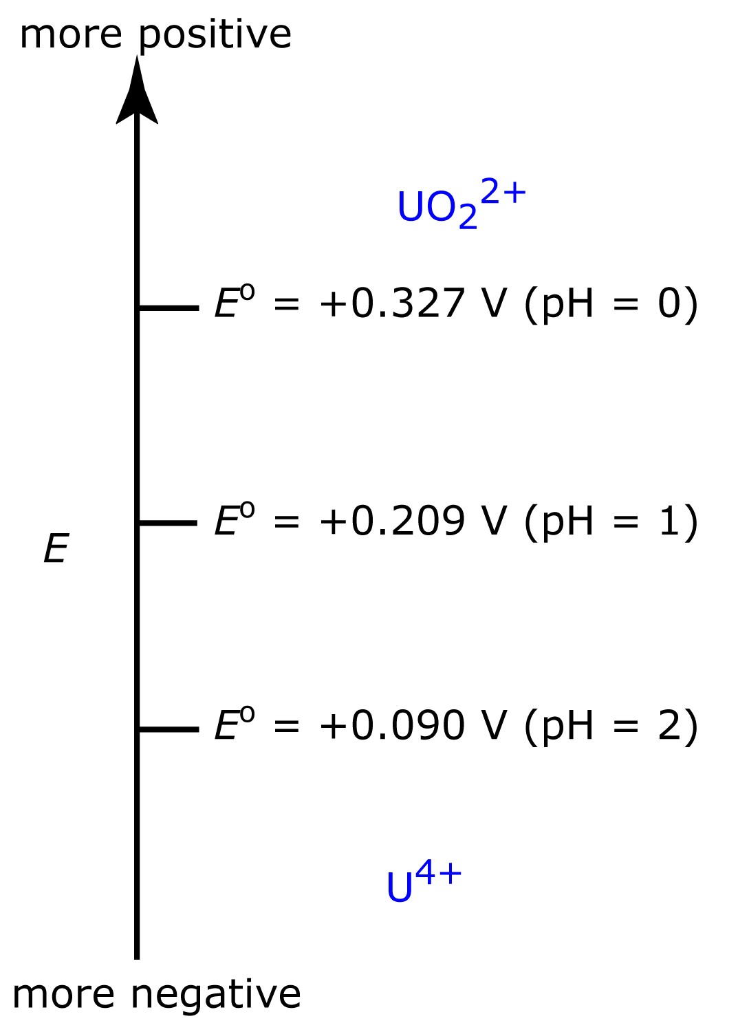
Figure 6.11 Redox ladder diagram for the UO₂²⁺/U⁴⁺ half-reaction showing the effect of pH on the step.

Contributors

• David Harvey (DePauw University)