
Spherical Harmonics
- Page ID
- 64932
Spherical Harmonics are a group of functions used in math and the physical sciences to solve problems in disciplines including geometry, partial differential equations, and group theory. The general, normalized Spherical Harmonic is depicted below:
\[ Y_{l}^{m}(\theta,\phi) = \sqrt{ \dfrac{(2l + 1)(l - |m|)!}{4\pi (l + |m|)!} } P_{l}^{|m|}(\cos\theta)e^{im\phi} \]
One of the most prevalent applications for these functions is in the description of angular quantum mechanical systems.
Utilized first by Laplace in 1782, these functions did not receive their name until nearly ninety years later by Lord Kelvin. Any harmonic is a function that satisfies Laplace's differential equation:
\[ \nabla^2 \psi = 0 \]
These harmonics are classified as spherical due to being the solution to the angular portion of Laplace's equation in the spherical coordinate system. Laplace's work involved the study of gravitational potentials and Kelvin used them in a collaboration with Peter Tait to write a textbook. In the 20th century, Erwin Schrödinger and Wolfgang Pauli both released papers in 1926 with details on how to solve the "simple" hydrogen atom system. Now, another ninety years later, the exact solutions to the hydrogen atom are still used to analyze multi-electron atoms and even entire molecules. Much of modern physical chemistry is based around framework that was established by these quantum mechanical treatments of nature.
The "Basic" Description
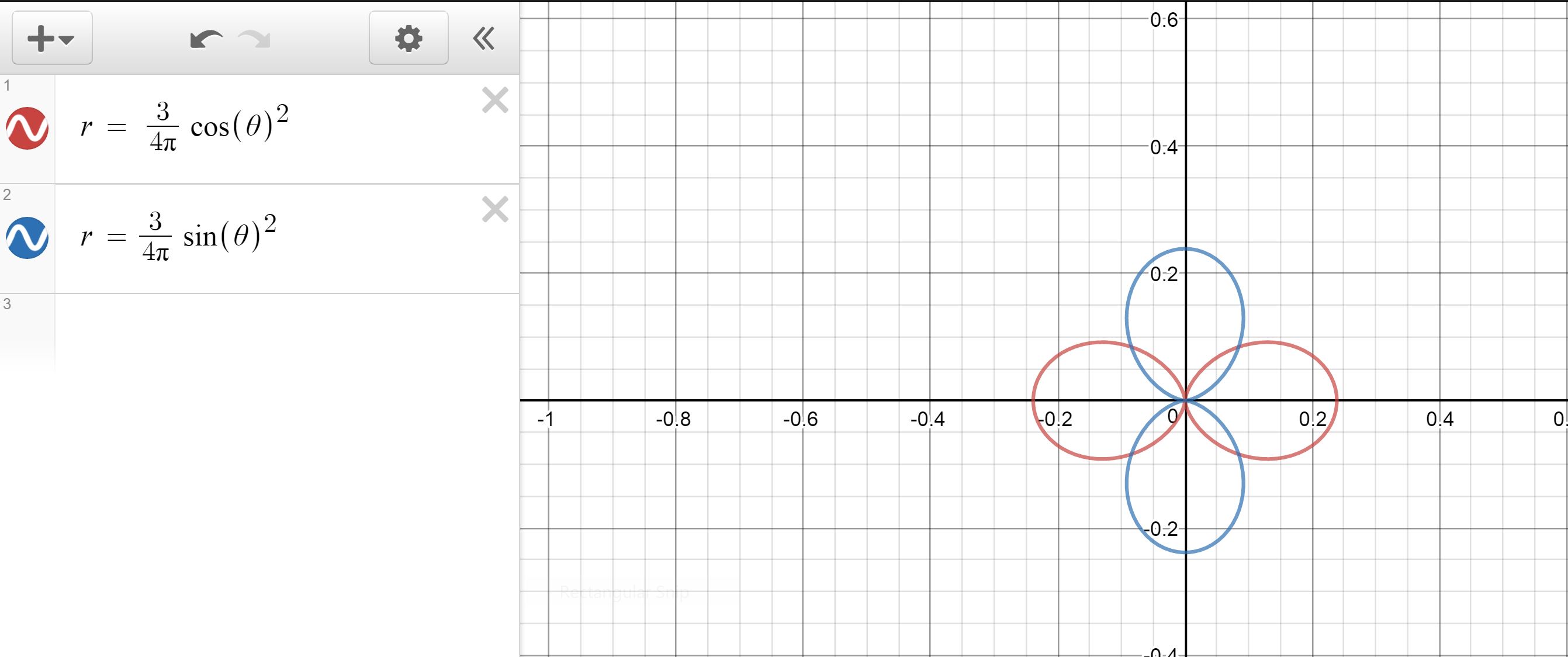
The 2px and 2pz (angular) probability distributions depicted on the left and graphed on the right using "desmos".
As Spherical Harmonics are unearthed by working with Laplace's equation in spherical coordinates, these functions are often products of trigonometric functions. These products are represented by the \( P_{l}^{|m|}(\cos\theta)\) term, which is called a Legendre polynomial. The details of where these polynomials come from are largely unnecessary here, lest we say that it is the set of solutions to a second differential equation that forms from attempting to solve Laplace's equation. Unsurprisingly, that equation is called "Legendre's equation", and it features a transformation of \(\cos\theta = x\). As the general function shows above, for the spherical harmonic where \(l = m = 0\), the bracketed term turns into a simple constant. The exponential equals one and we say that:
\[ Y_{0}^{0}(\theta,\phi) = \sqrt{ \dfrac{1}{4\pi} }\]
What is not shown in full is what happens to the Legendre polynomial attached to our bracketed expression. In the simple \(l = m = 0\) case, it disappears.
It is no coincidence that this article discusses both quantum mechanics and two variables, \(l\) and \(m\). These are exactly the angular momentum quantum number and magnetic quantum number, respectively, that are mentioned in General Chemistry classes. If we consider spectroscopic notation, an angular momentum quantum number of zero suggests that we have an s orbital if all of \(\psi(r,\theta,\phi)\) is present. This s orbital appears spherically symmetric on the boundary surface. In other words, the function looks like a ball. This is consistent with our constant-valued harmonic, for it would be constant-radius.
Extending these functions to larger values of \(l\) leads to increasingly intricate Legendre polynomials and their associated \(m\) values. The \({Y_{1}^{0}}^{*}Y_{1}^{0}\) and \({Y_{1}^{1}}^{*}Y_{1}^{1}\) functions are plotted above. Recall that these functions are multiplied by their complex conjugate to properly represent the Born Interpretation of "probability-density" (\(\psi^{*}\psi)\). It is also important to note that these functions alone are not referred to as orbitals, for this would imply that both the radial and angular components of the wavefunction are used.
Identify the location(s) of all planar nodes of the following spherical harmonic:
\[Y_{2}^{0}(\theta,\phi) = \sqrt{ \dfrac{5}{16\pi} }(3cos^2\theta - 1)\]
Solution
Nodes are points at which our function equals zero, or in a more natural extension, they are locations in the probability-density where the electron will not be found (i.e. \(\psi^{*}\psi = 0)\). As this specific function is real, we could square it to find our probability-density.
\[Y_{2}^{0} = [Y_{2}^{0}]^2 = 0\]
As the non-squared function will be computationally easier to work with, and will give us an equivalent answer, we do not bother to square the function. The constant in front can be divided out of the expression, leaving:
\[3cos^2\theta - 1 = 0\]
\[\theta = cos^{-1}\bigg[\pm\dfrac{1}{\sqrt3}\bigg]\]
\[\theta = 54.7^o \& 125.3^o\]
The Advanced Description
We have described these functions as a set of solutions to a differential equation but we can also look at Spherical Harmonics from the standpoint of operators and the field of linear algebra. For the curious reader, a more in depth treatment of Laplace's equation and the methods used to solve it in the spherical domain are presented in this section of the text. For a brief review, partial differential equations are often simplified using a separation of variables technique that turns one PDE into several ordinary differential equations (which is easier, promise). This allows us to say \(\psi(r,\theta,\phi) = R_{nl}(r)Y_{l}^{m}(\theta,\phi)\), and to form a linear operator that can act on the Spherical Harmonics in an eigenvalue problem. The more important results from this analysis include (1) the recognition of an \(\hat{L}^2\) operator and (2) the fact that the Spherical Harmonics act as an eigenbasis for the given vector space.
The \(\hat{L}^2\) operator is the operator associated with the square of angular momentum. It is directly related to the Hamiltonian operator (with zero potential) in the same way that kinetic energy and angular momentum are connected in classical physics.
\[\hat{H} = \dfrac{\hat{L}^2}{2I}\]
for \(I\) equal to the moment of inertia of the represented system. It is a linear operator (follows rules regarding additivity and homogeneity). More specifically, it is Hermitian. This means that when it is used in an eigenvalue problem, all eigenvalues will be real and the eigenfunctions will be orthogonal.
In Dirac notation, orthogonality means that the inner product of any two different eigenfunctions will equal zero:
\[\langle \psi_{i} | \psi_{j} \rangle = 0\]
When we consider the fact that these functions are also often normalized, we can write the classic relationship between eigenfunctions of a quantum mechanical operator using a piecewise function: the Kronecker delta.
\[\langle \psi_{i} | \psi_{j} \rangle = \delta_{ij} \, for \, \delta_{ij} = \begin{cases} 0 & i \neq j \ 1 & i = j \end{cases} \]
This relationship also applies to the spherical harmonic set of solutions, and so we can write an orthonormality relationship for each quantum number:
\[\langle Y_{l}^{m} | Y_{k}^{n} \rangle = \delta_{lk}\delta_{mn}\]
The parity operator is sometimes denoted by "P", but will be referred to as \(\Pi\) here to not confuse it with the momentum operator. When this Hermitian operator is applied to a function, the signs of all variables within the function flip. This operator gives us a simple way to determine the symmetry of the function it acts on.
Recall that even functions appear as \(f(x) = f(-x)\), and odd functions appear as \(f(-x) = -f(x)\). Combining this with \(\Pi\) gives the conditions:
- If \[\Pi Y_{l}^{m}(\theta,\phi) = Y_{l}^{m}(-\theta,-\phi)\] then the harmonic is even.
- If \[\Pi Y_{l}^{m}(\theta,\phi) = -Y_{l}^{m}(\theta,\phi)\] then the harmonic is odd.
Using the parity operator and properties of integration, determine \(\langle Y_{l}^{m}| Y_{k}^{n} \rangle\) for any \( l\) an even number and \(k\) an odd number.
Solution
As this question is for any even and odd pairing, the task seems quite daunting, but analyzing the parity for a few simple cases will lead to a dramatic simplification of the problem.
Start with acting the parity operator on the simplest spherical harmonic, \(l = m = 0\):
\[\Pi Y_{0}^{0}(\theta,\phi) = \sqrt{\dfrac{1}{4\pi}} = Y_{0}^{0}(-\theta,-\phi)\]
Now we can scale this up to the \(Y_{2}^{0}(\theta,\phi)\) case given in example one:
\[\Pi Y_{2}^{0}(\theta,\phi) = \sqrt{ \dfrac{5}{16\pi} }(3cos^2(-\theta) - 1)\]
but cosine is an even function, so again, we see:
\[ Y_{2}^{0}(-\theta,-\phi) = Y_{2}^{0}(\theta,\phi)\]
It appears that for every even, angular QM number, the spherical harmonic is even. As it turns out, every odd, angular QM number yields odd harmonics as well! If this is the case (verified after the next example), then we now have a simple task ahead of us.
Note: Odd functions with symmetric integrals must be zero.
\[\langle Y_{l}^{m}| Y_{k}^{n} \rangle = \int_{-\inf}^{\inf} (EVEN)(ODD)d\tau \]
An even function multiplied by an odd function is an odd function (like even and odd numbers when multiplying them together). As such, this integral will be zero always, no matter what specific \(l\) and \(k\) are used. As one can imagine, this is a powerful tool. The impact is lessened slightly when coming off the heels off the idea that Hermitian operators like \(\hat{L}^2\) yield orthogonal eigenfunctions, but general parity of functions is useful!
Consider the question of wanting to know the expectation value of our colatitudinal coordinate \(\theta\) for any given spherical harmonic with even-\(l\).
\[\langle \theta \rangle = \langle Y_{l}^{m} | \theta | Y_{l}^{m} \rangle \]
\[\langle \theta \rangle = \int_{-\inf}^{\inf} (EVEN)(ODD)(EVEN)d\tau \]
Again, a complex sounding problem is reduced to a very straightforward analysis. Using integral properties, we see this is equal to zero, for any even-\(l\).
.JPG?revision=1) |
.JPG?revision=1) |
A photo-set reminder of why an eigenvector (blue) is special. From https://en.Wikipedia.org/wiki/Eigenvalues_and_eigenvectors.
Lastly, the Spherical Harmonics form a complete set, and as such can act as a basis for the given (Hilbert) space. This means any spherical function can be written as a linear combination of these basis functions, (for the basis spans the space of continuous spherical functions by definition):
\[f(\theta,\phi) = \sum_{l}\sum_{m} \alpha_{lm} Y_{l}^{m}(\theta,\phi) \]
While any particular basis can act in this way, the fact that the Spherical Harmonics can do this shows a nice relationship between these functions and the Fourier Series, a basis set of sines and cosines. Spherical Harmonics are considered the higher-dimensional analogs of these Fourier combinations, and are incredibly useful in applications involving frequency domains. In the past few years, with the advancement of computer graphics and rendering, modeling of dynamic lighting systems have led to a new use for these functions.
In order to do any serious computations with a large sum of Spherical Harmonics, we need to be able to generate them via computer in real-time (most specifically for real-time graphics systems). This requires the use of either recurrence relations or generating functions. While at the very top of this page is the general formula for our functions, the Legendre polynomials are still as of yet undefined. The two major statements required for this example are listed:
\( P_{l}(x) = \dfrac{1}{2^{l}l!} \dfrac{d^{l}}{dx^{l}}[(x^{2} - 1)^{l}]\)
\( P_{l}^{|m|}(x) = (1 - x^{2})^{\tiny\dfrac{|m|}{2}}\dfrac{d^{|m|}}{dx^{|m|}}P_{l}(x)\)
Using these recurrence relations, write the spherical harmonic \(Y_{1}^{1}(\theta,\phi)\).
Solution
To solve this problem, we can break up our process into four major parts. The first is determining our \(P_{l}(x)\) function. As \(l = 1\):
\( P_{1}(x) = \dfrac{1}{2^{1}1!} \dfrac{d}{dx}[(x^{2} - 1)]\)
\( P_{1}(x) = \dfrac{1}{2}(2x)\)
\( P_{1}(x) = x\)
Now that we have \(P_{l}(x)\), we can plug this into our Legendre recurrence relation to find the associated Legendre function, with \(m = 1\):
\( P_{1}^{1}(x) = (1 - x^{2})^{\tiny\dfrac{1}{2}}\dfrac{d}{dx}x\)
\( P_{1}^{1}(x) = (1 - x^{2})^{\tiny\dfrac{1}{2}}\)
At the halfway point, we can use our general definition of Spherical Harmonics with the newly determined Legendre function. With \(m = l = 1\):
\[ Y_{1}^{1}(\theta,\phi) = \sqrt{ \dfrac{(2(1) + 1)(1 - 1)!}{4\pi (1 + |1|)!} } (1 - x^{2})^{\tiny\dfrac{1}{2}}e^{i\phi} \]
\[ Y_{1}^{1}(\theta,\phi) = \sqrt{ \dfrac{3}{8\pi} } (1 - x^{2})^{\tiny\dfrac{1}{2}}e^{i\phi} \]
The last step is converting our Cartesian function into the proper coordinate system or making the switch from x to \(\cos\theta\).
\[ Y_{1}^{1}(\theta,\phi) = \sqrt{ \dfrac{3}{8\pi} } (1 - (\cos\theta)^{2})^{\tiny\dfrac{1}{2}}e^{i\phi} \]
\[ Y_{1}^{1}(\theta,\phi) = \sqrt{ \dfrac{3}{8\pi} } (sin^{2}\theta)^{\tiny\dfrac{1}{2}}e^{i\phi} \]
\[ Y_{1}^{1}(\theta,\phi) = \sqrt{ \dfrac{3}{8\pi} }sin\theta e^{i\phi} \]
As a side note, there are a number of different relations one can use to generate Spherical Harmonics or Legendre polynomials. Often times, efficient computer algorithms have much longer polynomial terms than the short, derivative-based statements from the beginning of this problem.
As a final topic, we should take a closer look at the two recursive relations of Legendre polynomials together. As derivatives of even functions yield odd functions and vice versa, we note that for our first equation, an even \(l\) value implies an even number of derivatives, and this will yield another even function. When we plug this into our second relation, we now have to deal with \(|m|\) derivatives of our \(P_{l}\) function. We are in luck though, as in the spherical harmonic functions there is a separate component entirely dependent upon the sign of \(m\). As such, any changes in parity to the Legendre polynomial (to create the associated Legendre function) will be undone by the flip in sign of \(m\) in the azimuthal component. Parity only depends on \(l\)!
This confirms our prediction from the second example that any Spherical Harmonic with even-\(l\) is also even, and any odd-\(l\) leads to odd \(Y_{l}^{m}\).
References
- Details on the History of S.H. - http://www.liquisearch.com/spherical_harmonics/history
- A collection of Schrödinger's papers, dated 1926 - http://www.physics.drexel.edu/~bob/Quantum_Papers/Schr_1.pdf
- Details on Kelvin and Tait's Collaboration - http://www.oxfordscholarship.com/view/10.1093/acprof:oso/9780199231256.001.0001/acprof-9780199231256-chapter-11
- Graph \(\theta\) Traces of S.H. Functions with Desmos - https://www.desmos.com/
- Information on Hermitian Operators - www.pa.msu.edu/~mmoore/Lect4_BasisSet.pdf
- Discussions of S.H. Functions and Computer Graphics - www.cs.dartmouth.edu/~wjarosz/publications/dissertation/appendixB.pdf and http://www.cs.columbia.edu/~dhruv/lighting.pdf
Contributors and Attributions
- Alexander Staat