
3.1.2: Maxwell-Boltzmann Distributions
- Page ID
- 1407
The Maxwell-Boltzmann equation, which forms the basis of the kinetic theory of gases, defines the distribution of speeds for a gas at a certain temperature. From this distribution function, the most probable speed, the average speed, and the root-mean-square speed can be derived.
Introduction
The kinetic molecular theory is used to determine the motion of a molecule of an ideal gas under a certain set of conditions. However, when looking at a mole of ideal gas, it is impossible to measure the velocity of each molecule at every instant of time. Therefore, the Maxwell-Boltzmann distribution is used to determine how many molecules are moving between velocities \(v\) and \(v + dv\). Assuming that the one-dimensional distributions are independent of one another, that the velocity in the y and z directions does not affect the x velocity, for example, the Maxwell-Boltzmann distribution is given by
\[ \dfrac{dN}{N}= \left(\frac{m}{2\pi k_BT} \right)^{1/2}e^{\frac{-mv^2}{2k_BT}}dv \label{1} \]
where
- \(dN/N\) is the fraction of molecules moving at velocity \(v\) to \(v + dv\),
- \(m\) is the mass of the molecule,
- \(k_b\) is the Boltzmann constant, and
- \(T\) is the absolute temperature.1
Additionally, the function can be written in terms of the scalar quantity speed c instead of the vector quantity velocity. This form of the function defines the distribution of the gas molecules moving at different speeds, between \(c_1\) and \(c_2\), thus
\[f(c)=4\pi c^2 \left (\frac{m}{2\pi k_BT} \right)^{3/2}e^{\frac{-mc^2}{2k_BT}} \label{2} \]
Finally, the Maxwell-Boltzmann distribution can be used to determine the distribution of the kinetic energy of for a set of molecules. The distribution of the kinetic energy is identical to the distribution of the speeds for a certain gas at any temperature.2
Plotting the Maxwell-Boltzmann Distribution Function
Figure 1 shows the Maxwell-Boltzmann distribution of speeds for a certain gas at a certain temperature, such as nitrogen at 298 K. The speed at the top of the curve is called the most probable speed because the largest number of molecules have that speed.
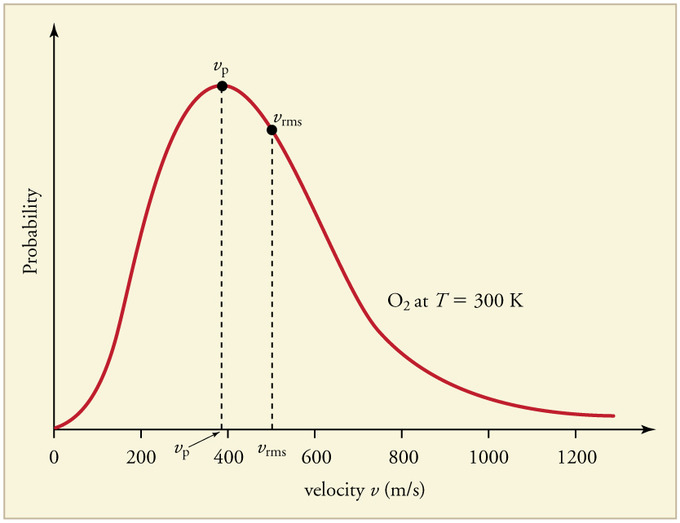
Figure 2 shows how the Maxwell-Boltzmann distribution is affected by temperature. At lower temperatures, the molecules have less energy. Therefore, the speeds of the molecules are lower and the distribution has a smaller range. As the temperature of the molecules increases, the distribution flattens out. Because the molecules have greater energy at higher temperature, the molecules are moving faster.

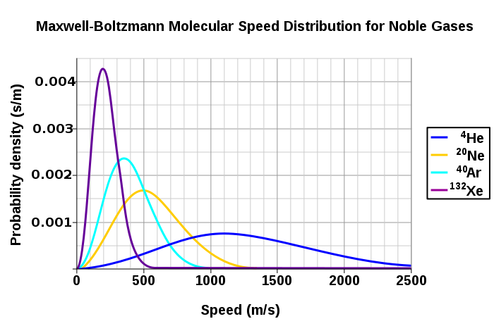
Figure 3 shows the dependence of the Maxwell-Boltzmann distribution on molecule mass. On average, heavier molecules move more slowly than lighter molecules. Therefore, heavier molecules will have a smaller speed distribution, while lighter molecules will have a speed distribution that is more spread out.
Related Speed Expressions
Three speed expressions can be derived from the Maxwell-Boltzmann distribution: the most probable speed, the average speed, and the root-mean-square speed. The most probable speed is the maximum value on the distribution plot. This is established by finding the velocity when the following derivative is zero
\[\dfrac{df(c)}{dc}|_{C_{mp}} = 0 \nonumber \]
which is
\[C_{mp}=\sqrt {\dfrac {2RT}{M}} \label{3a} \]
The average speed is the sum of the speeds of all the molecules divided by the number of molecules.
\[C_{avg}=\int_0^{\infty} c f(c) dc = \sqrt {\dfrac{8RT}{\pi M}} \label{3b} \]
The root-mean-square speed is square root of the average speed-squared.
\[ C_{rms}=\sqrt {\dfrac {3RT}{M}} \label{3c} \]
where
- \(R\) is the gas constant,
- \(T\) is the absolute temperature and
- \(M\) is the molar mass of the gas.
It always follows that for gases that follow the Maxwell-Boltzmann distribution (if thermallized)
\[C_{mp}< C_{avg}< C_{rms} \label{4} \]
References
- Dunbar, R.C. Deriving the Maxwell Distribution J. Chem. Ed. 1982, 59, 22-23.
- Peckham, G.D.; McNaught, I.J.; Applications of the Maxwell-Boltzmann Distribution J. Chem. Ed. 1992, 69, 554-558.
- Chang, R. Physical Chemistry for the Biosciences, 25-27.
Problems
- Using the Maxwell-Boltzman function, calculate the fraction of argon gas molecules with a speed of 305 m/s at 500 K.
- If the system in problem 1 has 0.46 moles of argon gas, how many molecules have the speed of 305 m/s?
- Calculate the values of \(C_{mp}\), \(C_{avg}\), and \(C_{rms}\) for xenon gas at 298 K.
- From the values calculated above, label the Boltzmann distribution plot (Figure 1) with the approximate locations of (C_{mp}\), \(C_{avg}\), and \(C_{rms}\).
- What will have a larger speed distribution, helium at 500 K or argon at 300 K? Helium at 300 K or argon at 500 K? Argon at 400 K or argon at 1000 K?
Answers
1. 0.00141
2. \(3.92 \times 10^{20}\) argon molecules
3. Cmp = 194.27 m/s
Cavg = 219.21 m/s
Crms = 237.93 m/s
4. As stated above, Cmp is the most probable speed, thus it will be at the top of the distribution curve. To the right of the most probable speed will be the average speed, followed by the root-mean-square speed.
5. Hint: Use the related speed expressions to determine the distribution of the gas molecules: helium at 500 K. helium at at 300 K. argon at 1000 K.