
6.4.1: Eyring equation
- Page ID
- 1395
The Eyring Equation, developed by Henry Eyring in 1935, is based on transition state theory and is used to describe the relationship between reaction rate and temperature. It is similar to the Arrhenius Equation, which also describes the temperature dependence of reaction rates. However, whereas Arrhenius Equation can be applied only to gas-phase kinetics, the Eyring Equation is useful in the study of gas, condensed, and mixed-phase reactions that have no relevance to the collision model.
Introduction
The Eyring Equation gives a more accurate calculation of rate constants and provides insight into how a reaction progresses at the molecular level. The Equation is given below:
\[ k = \dfrac{k_BT}{h}e^{-\left ( \frac{\bigtriangleup H^\ddagger}{RT} \right )}e^{ \left ( \frac{\bigtriangleup S^\ddagger}{R} \right )} \label{1} \]
Consider a bimolecular reaction:
\[A~+B~\rightarrow~C \label{2} \]
\[K = \dfrac{[C]}{[A][B]} \label{3} \]
where \(K\) is the equilibrium constant. In the transition state model, the activated complex AB is formed:
\[A~+~B~\rightleftharpoons ~AB^\ddagger~\rightarrow ~C \label{4} \]
\[K^\ddagger=\dfrac{[AB]^\ddagger}{[A][B]} \label{5} \]
There is an energy barrier, called activation energy, in the reaction pathway. A certain amount of energy is required for the reaction to occur. The transition state, \(AB^\ddagger\), is formed at maximum energy. This high-energy complex represents an unstable intermediate. Once the energy barrier is overcome, the reaction is able to proceed and product formation occurs.
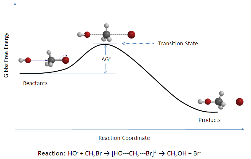
The rate of a reaction is equal to the number of activated complexes decomposing to form products. Hence, it is the concentration of the high-energy complex multiplied by the frequency of it surmounting the barrier.
\[\begin{eqnarray} rate~&=&~v[AB^\ddagger] \label{6} \\ &=&~v[A][B]K^\ddagger \label{7} \end{eqnarray} \]
The rate can be rewritten:
\[rate~=~k[A][B] \label{8} \]
Combining Equations \(\ref{8}\) and \(\ref{7}\) gives:
\[ \begin{eqnarray} k[A][B]~&=&~v[A][B]K^\ddagger \label{9} \\ k~&=&~vK^\ddagger \label{10} \end{eqnarray} \]
where
- \(v\) is the frequency of vibration,
- \(k\) is the rate constant and
- \(K ^\ddagger \) is the thermodynamic equilibrium constant.
The frequency of vibration is given by:
\[v~=~\dfrac{k_BT}{h} \label{11} \]
where
- \(k_B\) is the Boltzmann's constant (1.381 x 10⁻²³ J/K),
- \(T\) is the absolute temperature in Kelvin (K) and
- \(h\) is Planck's constant (6.626 x 10⁻³⁴ Js).
Substituting Equation \(\ref{11}\) into Equation \(\ref{10}\) :
\[k~=~\dfrac{k_BT}{h}K^\ddagger \label{12} \]
Equation \({ref}\) is often tagged with another term \((M^{1-m})\) that makes the units equal with \(M\) is the molarity and \(m\) is the molecularly of the reaction.
\[k~=~\dfrac{k_BT}{h}K^\ddagger (M^{1-m}) \label{E12} \]
The following thermodynamic equations further describe the equilibrium constant:
\[ \begin{eqnarray} \Delta G^\ddagger~&=&~-RT\ln{K^\ddagger}\label{13} \\ \Delta G^\ddagger~&=&~\Delta H^\ddagger~-~T\Delta S^\ddagger \label{14} \end{eqnarray} \]
where \(\Delta G^\ddagger\) is the Gibbs energy of activation, \(\Delta H^\ddagger\) is the enthalpy of activation and \(\Delta S^\ddagger\) is the entropy of activation. Combining Equations \(\ref{10}\) and \(\ref{11}\) to solve for \(\ln K ^\ddagger \) gives:
\[\ln{K}^\ddagger~=~-\dfrac{\Delta H^\ddagger}{RT}~+~\dfrac{\Delta S^\ddagger}{R} \label{15} \]
The Eyring Equation is finally given by substituting Equation \(\ref{15}\) into Equation \(\ref{12}\):
\[ k~=~\dfrac{k_BT}{h}e^{-\frac{\Delta H^\ddagger}{RT}}e^\frac{\Delta S^\ddagger}{R} \label{16} \]
Application of the Eyring Equation
The linear form of the Eyring Equation is given below:
\[\ln{\dfrac{k}{T}}~=~\dfrac{-\Delta H^\dagger}{R}\dfrac{1}{T}~+~\ln{\dfrac{k_B}{h}}~+~\dfrac{\Delta S^\ddagger}{R} \label{17} \]
The values for \(\Delta H^\ddagger\) and \(\Delta S^\ddagger\) can be determined from kinetic data obtained from a \(\ln{\dfrac{k}{T}}\) vs. \(\dfrac{1}{T}\) plot. The Equation is a straight line with negative slope, \(\dfrac{-\Delta H^\ddagger}{R}\), and a y-intercept, \(\dfrac{\Delta S^\ddagger}{R}+\ln{\dfrac{k_B}{h}}\).
References
- Chang, Raymond. Physical Chemistry for the Biosciences. USA: University Science Books, 2005. Page 338-342.
Contributors and Attributions
- Kelly Louie